Chapter 1 Why Statistics?
To call in statisticians after the experiment is done may be no more than asking them to perform a post-mortem examination: They may be able to say what the experiment died of. —Sir Ronald Fisher
1.1 On the psychology of statistics
Adapted nearly verbatim from Chapters 1 and 2 in Navarro, D. “Learning Statistics with R.” https://compcogscisydney.org/learning-statistics-with-r/
To the surprise of many students, statistics is a fairly significant part of a psychological education. To the surprise of no-one, statistics is very rarely the favorite part of one’s psychological education. After all, if you really loved the idea of doing statistics, you’d probably be enrolled in a statistics class right now, not a psychology class. So, not surprisingly, there’s a pretty large proportion of the student base that isn’t happy about the fact that psychology has so much statistics in it. In view of this, I thought that the right place to start might be to answer some of the more common questions that people have about stats…
A big part of this issue at hand relates to the very idea of statistics. What is it? What’s it there for? And why are scientists so bloody obsessed with it? These are all good questions, when you think about it. So let’s start with the last one. As a group, scientists seem to be bizarrely fixated on running statistical tests on everything. In fact, we use statistics so often that we sometimes forget to explain to people why we do. It’s a kind of article of faith among scientists – and especially social scientists – that your findings can’t be trusted until you’ve done some stats. Undergraduate students might be forgiven for thinking that we’re all completely mad, because no-one takes the time to answer one very simple question:
Why do you do statistics? Why don’t scientists just use common sense?
It’s a naive question in some ways, but most good questions are. There’s a lot of good answers to it, but for my money, the best answer is a really simple one: we don’t trust ourselves enough. We worry that we’re human, and susceptible to all of the biases, temptations and frailties that humans suffer from. Much of statistics is basically a safeguard. Using “common sense” to evaluate evidence means trusting gut instincts, relying on verbal arguments and on using the raw power of human reason to come up with the right answer. Most scientists don’t think this approach is likely to work.
In fact, come to think of it, this sounds a lot like a psychological question to me, and since I do work in a psychology department, it seems like a good idea to dig a little deeper here. Is it really plausible to think that this “common sense” approach is very trustworthy? Verbal arguments have to be constructed in language, and all languages have biases – some things are harder to say than others, and not necessarily because they’re false (e.g., quantum electrodynamics is a good theory, but hard to explain in words). The instincts of our “gut” aren’t designed to solve scientific problems, they’re designed to handle day to day inferences – and given that biological evolution is slower than cultural change, we should say that they’re designed to solve the day to day problems for a different world than the one we live in. Most fundamentally, reasoning sensibly requires people to engage in “induction”, making wise guesses and going beyond the immediate evidence of the senses to make generalisations about the world. If you think that you can do that without being influenced by various distractors, well, I have a bridge in Brooklyn I’d like to sell you. Heck, as the next section shows, we can’t even solve “deductive” problems (ones where no guessing is required) without being influenced by our pre-existing biases.
1.1.1 The curse of belief bias
People are mostly pretty smart. We’re certainly smarter than the other species that we share the planet with (though many people might disagree). Our minds are quite amazing things, and we seem to be capable of the most incredible feats of thought and reason. That doesn’t make us perfect though. And among the many things that psychologists have shown over the years is that we really do find it hard to be neutral, to evaluate evidence impartially and without being swayed by pre-existing biases. A good example of this is the belief bias effect in logical reasoning: if you ask people to decide whether a particular argument is logically valid (i.e., conclusion would be true if the premises were true), we tend to be influenced by the believability of the conclusion, even when we shouldn’t. For instance, here’s a valid argument where the conclusion is believable:
- No cigarettes are inexpensive (Premise 1)
- Some addictive things are inexpensive (Premise 2)
- Therefore, some addictive things are not cigarettes (Conclusion)
And here’s a valid argument where the conclusion is not believable:
- No addictive things are inexpensive (Premise 1)
- Some cigarettes are inexpensive (Premise 2)
- Therefore, some cigarettes are not addictive (Conclusion)
The logical structure of argument #2 is identical to the structure of argument #1, and they’re both valid. However, in the second argument, there are good reasons to think that premise 1 is incorrect, and as a result it’s probably the case that the conclusion is also incorrect. But that’s entirely irrelevant to the topic at hand: an argument is deductively valid if the conclusion is a logical consequence of the premises. That is, a valid argument doesn’t have to involve true statements.
On the other hand, here’s an invalid argument that has a believable conclusion:
- No addictive things are inexpensive (Premise 1)
- Some cigarettes are inexpensive (Premise 2)
- Therefore, some addictive things are not cigarettes (Conclusion)
And finally, an invalid argument with an unbelievable conclusion:
- No cigarettes are inexpensive (Premise 1)
- Some addictive things are inexpensive (Premise 2)
- Therefore, some cigarettes are not addictive (Conclusion)
Now, suppose that people really are perfectly able to set aside their pre-existing biases about what is true and what isn’t, and purely evaluate an argument on its logical merits. We’d expect 100% of people to say that the valid arguments are valid, and 0% of people to say that the invalid arguments are valid. So if you ran an experiment looking at this, you’d expect to see data like this:
| conclusion feels true | conclusion feels false | |
|---|---|---|
| argument is valid | 100% say “valid” | 100% say “valid” |
| argument is invalid | 0% say “valid” | 0% say “valid” |
If the psychological data looked like this (or even a good approximation to this), we might feel safe in just trusting our gut instincts. That is, it’d be perfectly okay just to let scientists evaluate data based on their common sense, and not bother with all this murky statistics stuff. However, you guys have taken psych classes, and by now you probably know where this is going.
In a classic study, Evans, Barston, and Pollard (1983) ran an experiment looking at exactly this. What they found is that when pre-existing biases (i.e., beliefs) were in agreement with the structure of the data, everything went the way you’d hope:
| conclusion feels true | conclusion feels false | |
|---|---|---|
| argument is valid | 92% say “valid” | – |
| argument is invalid | – | 8% say “valid” |
Not perfect, but that’s pretty good. But look what happens when our intuitive feelings about the truth of the conclusion run against the logical structure of the argument:
| conclusion feels true | conclusion feels false | |
|---|---|---|
| argument is valid | 92% say “valid” | 46% say “valid” |
| argument is invalid | 92% say “valid” | 8% say “valid” |
Oh dear, that’s not as good. Apparently, when people are presented with a strong argument that contradicts our pre-existing beliefs, we find it pretty hard to even perceive it to be a strong argument (people only did so 46% of the time). Even worse, when people are presented with a weak argument that agrees with our pre-existing biases, almost no-one can see that the argument is weak (people got that one wrong 92% of the time!)
If you think about it, it’s not as if these data are horribly damning. Overall, people did do better than chance at compensating for their prior biases, since about 60% of people’s judgements were correct (you’d expect 50% by chance). Even so, if you were a professional “evaluator of evidence”, and someone came along and offered you a magic tool that improves your chances of making the right decision from 60% to (say) 95%, you’d probably jump at it, right? Of course you would. Thankfully, we actually do have a tool that can do this. But it’s not magic, it’s statistics. So that’s reason #1 why scientists love statistics. It’s just too easy for us to “believe what we want to believe”; so if we want to “believe in the data” instead, we’re going to need a bit of help to keep our personal biases under control. That’s what statistics does: it helps keep us honest.
1.2 The cautionary tale of Simpson’s paradox
The following is a true story (I think…). In 1973, the University of California, Berkeley had some worries about the admissions of students into their postgraduate courses. Specifically, the thing that caused the problem was that the gender breakdown of their admissions, which looked like this:
| Number of applicants | Percent admitted | |
| Men | 8442 | 44% |
| Women | 4321 | 35% |
and they were worried about being sued. Given that there were nearly 13,000 applicants, a difference of 9% in admission rates between men and women is just way too big to be a coincidence. Pretty compelling data, right? And if I were to say to you that these data actually reflect a weak bias in favour of women (sort of!), you’d probably think that I was either crazy or sexist.
Earlier versions of these notes incorrectly suggested that they actually were sued – apparently that’s not true. There’s a nice commentary on this here: https://www.refsmmat.com/posts/2016-05-08-simpsons-paradox-berkeley.html. A big thank you to Wilfried Van Hirtum for pointing this out to me!
When people started looking more carefully at the admissions data (Bickel, Hammel, and O’Connell 1975) they told a rather different story. Specifically, when they looked at it on a department by department basis, it turned out that most of the departments actually had a slightly higher success rate for woman applicants than for man applicants. The table below shows the admission figures for the six largest departments (with the names of the departments removed for privacy reasons):
| Men | Women | |||
| Department | Applicants | Percent admitted | Applicants | Percent admitted |
| A | 825 | 62% | 108 | 82% |
| B | 560 | 63% | 25 | 68% |
| C | 325 | 37% | 593 | 34% |
| D | 417 | 33% | 375 | 35% |
| E | 191 | 28% | 393 | 24% |
| F | 373 | 6% | 341 | 7% |
Remarkably, most departments had a higher rate of admissions for women than for men! Yet the overall rate of admission across the university for women was lower than for men How can this be? How can both of these statements be true at the same time?
Here’s what’s going on. Firstly, notice that the departments are not equal to one another in terms of their admission percentages: some departments (e.g., engineering, chemistry) tended to admit a high percentage of the qualified applicants, whereas others (e.g., English) tended to reject most of the candidates, even if they were high quality. So, among the six departments shown above, notice that department A is the most generous, followed by B, C, D, E and F in that order. Next, notice that men and women tended to apply to different departments. If we rank the departments in terms of the total number of man applicants, we get A\(>\)B\(>\)D\(>\)C\(>\)F\(>\)E (the “easy” departments are in bold). On the whole, men tended to apply to the departments that had high admission rates. Now compare this to how the woman applicants distributed themselves. Ranking the departments in terms of the total number of woman applicants produces a quite different ordering C\(>\)E\(>\)D\(>\)F\(>\)A\(>\)B. In other words, what these data seem to be suggesting is that the woman applicants tended to apply to “harder” departments. And in fact, if we look at all Figure 1.1 we see that this trend is systematic, and quite striking. This effect is known as Simpson’s paradox. It’s not common, but it does happen in real life, and most people are very surprised by it when they first encounter it, and many people refuse to even believe that it’s real. It is very real. And while there are lots of very subtle statistical lessons buried in there, I want to use it to make a much more important point. Doing research is hard, and there are lots of subtle, counterintuitive traps lying in wait for the unwary. That’s reason #2 why scientists love statistics, and why we teach research methods. Because science is hard, and the truth is sometimes cunningly hidden in the nooks and crannies of complicated data.
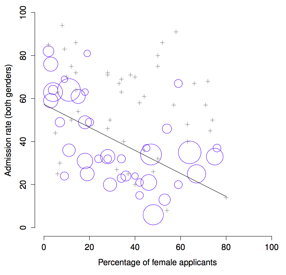
Figure 1.1: The Berkeley 1973 college admissions data. This figure plots the admission rate for the 85 departments that had at least one woman applicant, as a function of the percentage of applicants that were women. The plot is a redrawing of Figure 1 from Bickel et al. (1975). Circles plot departments with more than 40 applicants; the area of the circle is proportional to the total number of applicants. The crosses plot department with fewer than 40 applicants.
Before leaving this topic entirely, I want to point out something else really critical that is often overlooked in a research methods class. Statistics only solves part of the problem. Remember that we started all this with the concern that Berkeley’s admissions processes might be unfairly biased against woman applicants. When we looked at the “aggregated” data, it did seem like the university was discriminating against women, but when we “disaggregate” and looked at the individual behaviour of all the departments, it turned out that the actual departments were, if anything, slightly biased in favour of women. The gender bias in total admissions was caused by the fact that women tended to self-select for harder departments. From a legal perspective, that would probably put the university in the clear. Postgraduate admissions are determined at the level of the individual department (and there are good reasons to do that), and at the level of individual departments, the decisions are more or less unbiased (the weak bias in favour of women at that level is small, and not consistent across departments). Since the university can’t dictate which departments people choose to apply to, and the decision making takes place at the level of the department it can hardly be held accountable for any biases that those choices produce.
That was the basis for my somewhat glib remarks earlier, but that’s not exactly the whole story, is it? After all, if we’re interested in this from a more sociological and psychological perspective, we might want to ask why there are such strong gender differences in applications. Why do men tend to apply to engineering more often than women, and why is this reversed for the English department? And why is it the case that the departments that tend to have an application bias towards women tend to have lower overall admission rates than those departments that have an application bias towards men? Might this not still reflect a gender bias, even though every single department is itself unbiased? It might. Suppose, hypothetically, that men preferred to apply to “hard sciences” and women prefer “humanities”. And suppose further that the reason for why the humanities departments have low admission rates is because the government doesn’t want to fund the humanities (spots in Ph.D. programs, for instance, are often tied to government funded research projects). Does that constitute a gender bias? Or just an unenlightened view of the value of the humanities? What if someone at a high level in the government cut the humanities funds because they felt that the humanities are “useless chick stuff”. That seems pretty blatantly gender biased. None of this falls within the purview of statistics, but it matters to the research project. If you’re interested in the overall structural effects of subtle gender biases, then you probably want to look at both the aggregated and disaggregated data. If you’re interested in the decision making process at Berkeley itself then you’re probably only interested in the disaggregated data.
In short there are a lot of critical questions that you can’t answer with statistics, but the answers to those questions will have a huge impact on how you analyse and interpret data. And this is the reason why you should always think of statistics as a tool to help you learn about your data, no more and no less. It’s a powerful tool to that end, but there’s no substitute for careful thought.
1.3 Statistics in psychology
I hope that the discussion above helped explain why science in general is so focused on statistics. But I’m guessing that you have a lot more questions about what role statistics plays in psychology, and specifically why psychology classes always devote so many lectures to stats. So here’s my attempt to answer a few of them…
- Why does psychology have so much statistics?
To be perfectly honest, there’s a few different reasons, some of which are better than others. The most important reason is that psychology is a statistical science. What I mean by that is that the “things” that we study are people. Real, complicated, gloriously messy, infuriatingly perverse people. The “things” of physics include objects like electrons, and while there are all sorts of complexities that arise in physics, electrons don’t have minds of their own. They don’t have opinions, they don’t differ from each other in weird and arbitrary ways, they don’t get bored in the middle of an experiment, and they don’t get angry at the experimenter and then deliberately try to sabotage the data set. At a fundamental level psychology is harder than physics.
Basically, we teach statistics to you as psychologists because you need to be better at stats than physicists. There’s actually a saying used sometimes in physics, to the effect that “if your experiment needs statistics, you should have done a better experiment”. They have the luxury of being able to say that because their objects of study are pathetically simple in comparison to the vast mess that confronts social scientists. It’s not just psychology, really: most social sciences are desperately reliant on statistics. Not because we’re bad experimenters, but because we’ve picked a harder problem to solve. We teach you stats because you really, really need it.
- Can’t someone else do the statistics?
To some extent, but not completely. It’s true that you don’t need to become a fully trained statistician just to do psychology, but you do need to reach a certain level of statistical competence. In my view, there’s three reasons that every psychological researcher ought to be able to do basic statistics:
There’s the fundamental reason: statistics is deeply intertwined with research design. If you want to be good at designing psychological studies, you need to at least understand the basics of stats.
If you want to be good at the psychological side of the research, then you need to be able to understand the psychological literature, right? But almost every paper in the psychological literature reports the results of statistical analyses. So if you really want to understand the psychology, you need to be able to understand what other people did with their data. And that means understanding a certain amount of statistics.
There’s a big practical problem with being dependent on other people to do all your statistics: statistical analysis is expensive. In almost any real life situation where you want to do psychological research, the cruel facts will be that you don’t have enough money to afford a statistician. So the economics of the situation mean that you have to be pretty self-sufficient.
Note that a lot of these reasons generalize beyond researchers. If you want to be a practicing psychologist and stay on top of the field, it helps to be able to read the scientific literature, which relies pretty heavily on statistics.
- I don’t care about jobs, research, or clinical work. Do I need statistics?
Okay, now you’re just messing with me. Still, I think it should matter to you too. Statistics should matter to you in the same way that statistics should matter to everyone: we live in the 21st century, and data are everywhere. Frankly, given the world in which we live these days, a basic knowledge of statistics is pretty damn close to a survival tool! Which is the topic of the next section…
1.4 Statistics in everyday life
“We are drowning in information,
but we are starved for knowledge”
– Various authors, original probably John Naisbitt
When I started writing up my lecture notes I took the 20 most recent news articles posted to the ABC news website. Of those 20 articles, it turned out that 8 of them involved a discussion of something that I would call a statistical topic; 6 of those made a mistake. The most common error, if you’re curious, was failing to report baseline data (e.g., the article mentions that 5% of people in situation X have some characteristic Y, but doesn’t say how common the characteristic is for everyone else!) The point I’m trying to make here isn’t that journalists are bad at statistics (though they almost always are), it’s that a basic knowledge of statistics is very helpful for trying to figure out when someone else is either making a mistake or even lying to you. Perhaps, one of the biggest things that a knowledge of statistics does to you is cause you to get angry at the newspaper or the internet on a far more frequent basis :).
1.5 There’s more to research methods than statistics
So far, most of what I’ve talked about is statistics, and so you’d be forgiven for thinking that statistics is all I care about in life. To be fair, you wouldn’t be far wrong, but research methodology is a broader concept than statistics. So most research methods courses will cover a lot of topics that relate much more to the pragmatics of research design, and in particular the issues that you encounter when trying to do research with humans. However, about 99% of student fears relate to the statistics part of the course, so I’ve focused on the stats in this discussion, and hopefully I’ve convinced you that statistics matters, and more importantly, that it’s not to be feared. That being said, it’s pretty typical for introductory research methods classes to be very stats-heavy. This is not (usually) because the lecturers are evil people. Quite the contrary, in fact. Introductory classes focus a lot on the statistics because you almost always find yourself needing statistics before you need the other research methods training. Why? Because almost all of your assignments in other classes will rely on statistical training, to a much greater extent than they rely on other methodological tools. It’s not common for undergraduate assignments to require you to design your own study from the ground up (in which case you would need to know a lot about research design), but it is common for assignments to ask you to analyse and interpret data that were collected in a study that someone else designed (in which case you need statistics). In that sense, from the perspective of allowing you to do well in all your other classes, the statistics is more urgent.
But note that “urgent” is different from “important” – they both matter. I really do want to stress that research design is just as important as data analysis, and this book does spend a fair amount of time on it. However, while statistics has a kind of universality, and provides a set of core tools that are useful for most types of psychological research, the research methods side isn’t quite so universal. There are some general principles that everyone should think about, but a lot of research design is very idiosyncratic, and is specific to the area of research that you want to engage in. To the extent that it’s the details that matter, those details don’t usually show up in an introductory stats and research methods class.
1.6 A brief introduction to research design
In this chapter, we’re going to start thinking about the basic ideas that go into designing a study, collecting data, checking whether your data collection works, and so on. It won’t give you enough information to allow you to design studies of your own, but it will give you a lot of the basic tools that you need to assess the studies done by other people. However, since the focus of this book is much more on data analysis than on data collection, I’m only giving a very brief overview. Note that this chapter is “special” in two ways. Firstly, it’s much more psychology-specific than the later chapters. Secondly, it focuses much more heavily on the scientific problem of research methodology, and much less on the statistical problem of data analysis. Nevertheless, the two problems are related to one another, so it’s traditional for stats textbooks to discuss the problem in a little detail. This chapter relies heavily on Campbell and Stanley (1963) for the discussion of study design, and Stevens (1946) for the discussion of scales of measurement. Later versions will attempt to be more precise in the citations.
1.7 Introduction to psychological measurement
The first thing to understand is data collection can be thought of as a kind of measurement. That is, what we’re trying to do here is measure something about human behaviour or the human mind. What do I mean by “measurement”?
1.7.1 Some thoughts about psychological measurement
Measurement itself is a subtle concept, but basically it comes down to finding some way of assigning numbers, or labels, or some other kind of well-defined descriptions to “stuff”. So, any of the following would count as a psychological measurement:
My age is 33 years.
I do not like anchovies.
My chromosomal sex is male.
My self-identified gender is a man.
In the short list above, the bolded part is “the thing to be measured”, and the italicized part is “the measurement itself”. In fact, we can expand on this a little bit, by thinking about the set of possible measurements that could have arisen in each case:
My age (in years) could have been 0, 1, 2, 3 …, etc. The upper bound on what my age could possibly be is a bit fuzzy, but in practice you’d be safe in saying that the largest possible age is 150, since no human has ever lived that long.
When asked if I like anchovies, I might have said that I do, or I do not, or I have no opinion, or I sometimes do.
My chromosomal sex is almost certainly going to be male (XY) or female (XX), but there are a few other possibilities. I could also have Klinfelter’s syndrome (XXY), which is more similar to male than to female. And I imagine there are other possibilities too.
My self-identified gender is also very likely to be a man or woman, but it doesn’t have to agree with my chromosomal sex. I may also identify with neither, or transgender, for example.
As you can see, for some things (like age) it seems fairly obvious what the set of possible measurements should be, whereas for other things it gets a bit tricky. But I want to point out that even in the case of someone’s age, it’s much more subtle than this. For instance, in the example above, I assumed that it was okay to measure age in years. But if you’re a developmental psychologist, that’s way too crude, and so you often measure age in years and months (if a child is 2 years and 11 months, this is usually written as “2;11”). If you’re interested in newborns, you might want to measure age in days since birth, maybe even hours since birth. In other words, the way in which you specify the allowable measurement values is important.
Looking at this a bit more closely, you might also realise that the concept of “age” isn’t actually all that precise. In general, when we say “age” we implicitly mean “the length of time since birth”. But that’s not always the right way to do it. Suppose you’re interested in how newborn babies control their eye movements. If you’re interested in kids that young, you might also start to worry that “birth” is not the only meaningful point in time to care about. If Baby Alice is born 3 weeks premature and Baby Bianca is born 1 week late, would it really make sense to say that they are the “same age” if we encountered them “2 hours after birth”? In one sense, yes: by social convention, we use birth as our reference point for talking about age in everyday life, since it defines the amount of time the person has been operating as an independent entity in the world, but from a scientific perspective that’s not the only thing we care about. When we think about the biology of human beings, it’s often useful to think of ourselves as organisms that have been growing and maturing since conception, and from that perspective Alice and Bianca aren’t the same age at all. So you might want to define the concept of “age” in two different ways: the length of time since conception, and the length of time since birth. When dealing with adults, it won’t make much difference, but when dealing with newborns it might.
Moving beyond these issues, there’s the question of methodology. What specific “measurement method” are you going to use to find out someone’s age? As before, there are lots of different possibilities:
You could just ask people “how old are you?” The method of self-report is fast, cheap and easy, but it only works with people old enough to understand the question, and some people lie about their age.
You could ask an authority (e.g., a parent) “how old is your child?” This method is fast, and when dealing with kids it’s not all that hard since the parent is almost always around. It doesn’t work as well if you want to know “age since conception”, since a lot of parents can’t say for sure when conception took place. For that, you might need a different authority (e.g., an obstetrician).
You could look up official records, like birth certificates. This is time consuming and annoying, but it has its uses (e.g., if the person is now dead).
1.7.2 Operationalization: defining your measurement
All of the ideas discussed in the previous section all relate to the concept of operationalization. To be a bit more precise about the idea, operationalization is the process by which we take a meaningful but somewhat vague concept, and turn it into a precise measurement. The process of operationalization can involve several different things:
Being precise about what you are trying to measure: For instance, does “age” mean “time since birth” or “time since conception” in the context of your research?
Determining what method you will use to measure it: Will you use self-report to measure age, ask a parent, or look up an official record? If you’re using self-report, how will you phrase the question?
Defining the set of the allowable values that the measurement can take: Note that these values don’t always have to be numerical, though they often are. When measuring age, the values are numerical, but we still need to think carefully about what numbers are allowed. Do we want age in years, years and months, days, hours? Etc. For other types of measurements (e.g., gender), the values aren’t numerical. But, just as before, we need to think about what values are allowed. If we’re asking people to self-report their gender, what options to we allow them to choose between? Is it enough to allow only “man” or “woman”? Do you need an “other” option? Or should we not give people any specific options, and let them answer in their own words? And if you open up the set of possible values to include all verbal response, how will you interpret their answers?
Operationalization is a tricky business, and there’s no “one, true way” to do it. The way in which you choose to operationalize the informal concept of “age” or “gender” into a formal measurement depends on what you need to use the measurement for. Often you’ll find that the community of scientists who work in your area have some fairly well-established ideas for how to go about it. In other words, operationalization needs to be thought through on a case by case basis. Nevertheless, while there a lot of issues that are specific to each individual research project, there are some aspects to it that are pretty general.
Before moving on, I want to take a moment to clear up our terminology, and in the process introduce one more term. Here are four different things that are closely related to each other:
A theoretical construct. This is the thing that you’re trying to take a measurement of, like “age”, “gender” or an “opinion”. A theoretical construct can’t be directly observed, and often they’re actually a bit vague.
A measure. The measure refers to the method or the tool that you use to make your observations. A question in a survey, a behavioural observation or a brain scan could all count as a measure.
An operationalization. The term “operationalization” refers to the logical connection between the measure and the theoretical construct, or to the process by which we try to derive a measure from a theoretical construct.
A variable. Finally, a new term. A variable is what we end up with when we apply our measure to something in the world. That is, variables are the actual “data” that we end up with in our data sets.
In practice, even scientists tend to blur the distinction between these things, but it’s very helpful to try to understand the differences.
1.8 Scales of measurement
As the previous section indicates, the outcome of a psychological measurement is called a variable. But not all variables are of the same qualitative type, and it’s very useful to understand what types there are. A very useful concept for distinguishing between different types of variables is what’s known as scales of measurement.
1.8.1 Nominal scale
A nominal scale variable (also referred to as a categorical variable) is one in which there is no particular relationship between the different possibilities: for these kinds of variables it doesn’t make any sense to say that one of them is ``bigger’ or “better” than any other one, and it absolutely doesn’t make any sense to average them. The classic example for this is “eye colour”. Eyes can be blue, green and brown, among other possibilities, but none of them is any “better” than any other one. As a result, it would feel really weird to talk about an “average eye colour”. Similarly, gender is nominal too: a man isn’t better or worse than a woman, neither does it make sense to try to talk about an “average gender”. In short, nominal scale variables are those for which the only thing you can say about the different possibilities is that they are different. That’s it.
Let’s take a slightly closer look at this. Suppose I was doing research on how people commute to and from work. One variable I would have to measure would be what kind of transportation people use to get to work. This “transport type” variable could have quite a few possible values, including: “train”, “bus”, “car”, “bicycle”, etc. For now, let’s suppose that these four are the only possibilities, and suppose that when I ask 100 people how they got to work today, and I get this:
| Transportation | Number of people |
|---|---|
| (1) Train | 12 |
| (2) Bus | 30 |
| (3) Car | 48 |
| (4) Bicycle | 10 |
So, what’s the average transportation type? Obviously, the answer here is that there isn’t one. It’s a silly question to ask. You can say that travel by car is the most popular method, and travel by train is the least popular method, but that’s about all. Similarly, notice that the order in which I list the options isn’t very interesting. I could have chosen to display the data like this and nothing really changes.
| Transportation | Number of people |
|---|---|
| (3) Car | 48 |
| (1) Train | 12 |
| (4) Bicycle | 10 |
| (2) Bus | 30 |
1.8.2 Ordinal scale
Ordinal scale variables have a bit more structure than nominal scale variables, but not by a lot. An ordinal scale variable is one in which there is a natural, meaningful way to order the different possibilities, but you can’t do anything else. The usual example given of an ordinal variable is “finishing position in a race”. You can say that the person who finished first was faster than the person who finished second, but you don’t know how much faster. As a consequence we know that 1st \(>\) 2nd, and we know that 2nd \(>\) 3rd, but the difference between 1st and 2nd might be much larger than the difference between 2nd and 3rd.
Here’s an more psychologically interesting example. Suppose I’m interested in people’s attitudes to climate change, and I ask them to pick one of these four statements that most closely matches their beliefs:
- Temperatures are rising, because of human activity
- Temperatures are rising, but we don’t know why
- Temperatures are rising, but not because of humans
- Temperatures are not rising
Notice that these four statements actually do have a natural ordering, in terms of “the extent to which they agree with the current science”. Statement 1 is a close match, statement 2 is a reasonable match, statement 3 isn’t a very good match, and statement 4 is in strong opposition to the science. So, in terms of the thing I’m interested in (the extent to which people endorse the science), I can order the items as \(1 > 2 > 3 > 4\). Since this ordering exists, it would be very weird to list the options like this…
- Temperatures are rising, but not because of humans
- Temperatures are rising, because of human activity
- Temperatures are not rising
- Temperatures are rising, but we don’t know why
…because it seems to violate the natural “structure” to the question.
So, let’s suppose I asked 100 people these questions, and got the following answers:
| Number | |
|---|---|
| (1) Temperatures are rising, because of human activity | 51 |
| (2) Temperatures are rising, but we don’t know why | 20 |
| (3) Temperatures are rising, but not because of humans | 10 |
| (4) Temperatures are not rising | 19 |
When analysing these data, it seems quite reasonable to try to group (1), (2) and (3) together, and say that 81 of 100 people were willing to at least partially endorse the science. And it’s also quite reasonable to group (2), (3) and (4) together and say that 49 of 100 people registered at least some disagreement with the dominant scientific view. However, it would be entirely bizarre to try to group (1), (2) and (4) together and say that 90 of 100 people said…what? There’s nothing sensible that allows you to group those responses together at all.
That said, notice that while we can use the natural ordering of these items to construct sensible groupings, what we can’t do is average them. For instance, in my simple example here, the “average” response to the question is 1.97. If you can tell me what that means, I’d love to know. Because that sounds like gibberish to me!
1.8.3 Interval scale
In contrast to nominal and ordinal scale variables, interval scale and ratio scale variables are variables for which the numerical value is genuinely meaningful. In the case of interval scale variables, the differences between the numbers are interpretable, but the variable doesn’t have a “natural” zero value. A good example of an interval scale variable is measuring temperature in degrees celsius. For instance, if it was 15\(^\circ\) yesterday and 18\(^\circ\) today, then the 3\(^\circ\) difference between the two is genuinely meaningful. Moreover, that 3\(^\circ\) difference is exactly the same as the 3\(^\circ\) difference between \(7^\circ\) and \(10^\circ\). In short, addition and subtraction are meaningful for interval scale variables.
However, notice that the \(0^\circ\) does not mean “no temperature at all”: it actually means “the temperature at which water freezes”, which is pretty arbitrary. As a consequence, it becomes pointless to try to multiply and divide temperatures. It is wrong to say that \(20^\circ\) is twice as hot as \(10^\circ\), just as it is weird and meaningless to try to claim that \(20^\circ\) is negative two times as hot as \(-10^\circ\).
Again, lets look at a more psychological example. Suppose I’m interested in looking at how the attitudes of first-year university students have changed over time. Obviously, I’m going to want to record the year in which each student started. This is an interval scale variable. A student who started in 2003 did arrive 5 years before a student who started in 2008. However, it would be completely insane for me to divide 2008 by 2003 and say that the second student started “1.0024 times later” than the first one. That doesn’t make any sense at all.
1.8.4 Ratio scale
The fourth and final type of variable to consider is a ratio scale variable, in which zero really means zero, and it’s okay to multiply and divide. A good psychological example of a ratio scale variable is response time (RT). In a lot of tasks it’s very common to record the amount of time somebody takes to solve a problem or answer a question, because it’s an indicator of how difficult the task is. Suppose that Alan takes 2.3 seconds to respond to a question, whereas Ben takes 3.1 seconds. As with an interval scale variable, addition and subtraction are both meaningful here. Ben really did take \(3.1 - 2.3 = 0.8\) seconds longer than Alan did. However, notice that multiplication and division also make sense here too: Ben took \(3.1 / 2.3 = 1.35\) times as long as Alan did to answer the question. And the reason why you can do this is that, for a ratio scale variable such as RT, “zero seconds” really does mean “no time at all”.
1.8.5 Continuous versus discrete variables
There’s a second kind of distinction that you need to be aware of, regarding what types of variables you can run into. This is the distinction between continuous variables and discrete variables. The difference between these is as follows:
A continuous variable is one in which, for any two values that you can think of, it’s always logically possible to have another value in between.
A discrete variable is, in effect, a variable that isn’t continuous. For a discrete variable, it’s sometimes the case that there’s nothing in the middle.
These definitions probably seem a bit abstract, but they’re pretty simple once you see some examples. For instance, response time is continuous. If Alan takes 3.1 seconds and Ben takes 2.3 seconds to respond to a question, then it’s possible for Cameron’s response time to lie in between, by taking 3.0 seconds. And of course it would also be possible for David to take 3.031 seconds to respond, meaning that his RT would lie in between Cameron’s and Alan’s. And while in practice it might be impossible to measure RT that precisely, it’s certainly possible in principle. Because we can always find a new value for RT in between any two other ones, we say that RT is continuous.
Discrete variables occur when this rule is violated. For example, nominal scale variables are always discrete: there isn’t a type of transportation that falls “in between” trains and bicycles, not in the strict mathematical way that 2.3 falls in between 2 and 3. So transportation type is discrete. Similarly, ordinal scale variables are always discrete: although “2nd place” does fall between “1st place” and “3rd place”, there’s nothing that can logically fall in between “1st place” and “2nd place”. Interval scale and ratio scale variables can go either way. As we saw above, response time (a ratio scale variable) is continuous. Temperature in degrees celsius (an interval scale variable) is also continuous. However, the year you went to school (an interval scale variable) is discrete. There’s no year in between 2002 and 2003. The number of questions you get right on a true-or-false test (a ratio scale variable) is also discrete: since a true-or-false question doesn’t allow you to be “partially correct”, there’s nothing in between 5/10 and 6/10. The table summarizes the relationship between the scales of measurement and the discrete/continuity distinction. Cells with a tick mark correspond to things that are possible. I’m trying to hammer this point home, because (a) some textbooks get this wrong, and (b) people very often say things like “discrete variable” when they mean “nominal scale variable”. It’s very unfortunate.
| continuous | discrete | |
|---|---|---|
| nominal | x | |
| ordinal | x | |
| interval | x | x |
| ratio | x | x |
1.8.6 Some complexities
Okay, I know you’re going to be shocked to hear this, but …the real world is much messier than this little classification scheme suggests. Very few variables in real life actually fall into these nice neat categories, so you need to be kind of careful not to treat the scales of measurement as if they were hard and fast rules. It doesn’t work like that: they’re guidelines, intended to help you think about the situations in which you should treat different variables differently. Nothing more.
So let’s take a classic example, maybe the classic example, of a psychological measurement tool: the Likert scale. The humble Likert scale is the bread and butter tool of all survey design. You yourself have filled out hundreds, maybe thousands of them, and odds are you’ve even used one yourself. Suppose we have a survey question that looks like this:
Which of the following best describes your opinion of the statement that “all pirates are freaking awesome” …
and then the options presented to the participant are these:
(1) Strongly disagree
(2) Disagree
(3) Neither agree nor disagree
(4) Agree
(5) Strongly agree
This set of items is an example of a 5-point Likert scale: people are asked to choose among one of several (in this case 5) clearly ordered possibilities, generally with a verbal descriptor given in each case. However, it’s not necessary that all items be explicitly described. This is a perfectly good example of a 5-point Likert scale too:
(1) Strongly disagree
(2)
(3)
(4)
(5) Strongly agree
Likert scales are very handy, if somewhat limited, tools. The question is, what kind of variable are they? They’re obviously discrete, since you can’t give a response of 2.5. They’re obviously not nominal scale, since the items are ordered; and they’re not ratio scale either, since there’s no natural zero.
But are they ordinal scale or interval scale? One argument says that we can’t really prove that the difference between “strongly agree” and “agree” is of the same size as the difference between “agree” and “neither agree nor disagree”. In fact, in everyday life it’s pretty obvious that they’re not the same at all. So this suggests that we ought to treat Likert scales as ordinal variables. On the other hand, in practice most participants do seem to take the whole “on a scale from 1 to 5” part fairly seriously, and they tend to act as if the differences between the five response options were fairly similar to one another. As a consequence, a lot of researchers treat Likert scale data as if it were interval scale. It’s not interval scale, but in practice it’s close enough that we usually think of it as being quasi-interval scale.
1.9 Assessing the reliability of a measurement
At this point we’ve thought a little bit about how to operationalize a theoretical construct and thereby create a psychological measure; and we’ve seen that by applying psychological measures we end up with variables, which can come in many different types. At this point, we should start discussing the obvious question: is the measurement any good? We’ll do this in terms of two related ideas: reliability and validity. Put simply, the reliability of a measure tells you how precisely you are measuring something, whereas the validity of a measure tells you how accurate the measure is.
Reliability is actually a very simple concept: it refers to the repeatability or consistency of your measurement. The measurement of my weight by means of a “bathroom scale” is very reliable: if I step on and off the scales over and over again, it’ll keep giving me the same answer. Measuring my intelligence by means of “asking my mom” is very unreliable: some days she tells me I’m a bit thick, and other days she tells me I’m a complete moron. Notice that this concept of reliability is different to the question of whether the measurements are correct (the correctness of a measurement relates to it’s validity). If I’m holding a sack of potatos when I step on and off of the bathroom scales, the measurement will still be reliable: it will always give me the same answer. However, this highly reliable answer doesn’t match up to my true weight at all, therefore it’s wrong. In technical terms, this is a reliable but invalid measurement. Similarly, while my mom’s estimate of my intelligence is a bit unreliable, she might be right. Maybe I’m just not too bright, and so while her estimate of my intelligence fluctuates pretty wildly from day to day, it’s basically right. So that would be an unreliable but valid measure. Of course, to some extent, notice that if my mum’s estimates are too unreliable, it’s going to be very hard to figure out which one of her many claims about my intelligence is actually the right one. To some extent, then, a very unreliable measure tends to end up being invalid for practical purposes; so much so that many people would say that reliability is necessary (but not sufficient) to ensure validity.
Okay, now that we’re clear on the distinction between reliability and validity, let’s have a think about the different ways in which we might measure reliability:
Test-retest reliability. This relates to consistency over time: if we repeat the measurement at a later date, do we get a the same answer?
Inter-rater reliability. This relates to consistency across people: if someone else repeats the measurement (e.g., someone else rates my intelligence) will they produce the same answer?
Parallel forms reliability. This relates to consistency across theoretically-equivalent measurements: if I use a different set of bathroom scales to measure my weight, does it give the same answer?
Internal consistency reliability. If a measurement is constructed from lots of different parts that perform similar functions (e.g., a personality questionnaire result is added up across several questions) do the individual parts tend to give similar answers.
Not all measurements need to possess all forms of reliability. For instance, educational assessment can be thought of as a form of measurement. One of the subjects that I teach, Computational Cognitive Science, has an assessment structure that has a research component and an exam component (plus other things). The exam component is intended to measure something different from the research component, so the assessment as a whole has low internal consistency. However, within the exam there are several questions that are intended to (approximately) measure the same things, and those tend to produce similar outcomes; so the exam on its own has a fairly high internal consistency. Which is as it should be. You should only demand reliability in those situations where you want to be measure the same thing!
1.10 The role of variables: predictors and outcomes
Okay, I’ve got one last piece of terminology that I need to explain to you before moving away from variables. Normally, when we do some research we end up with lots of different variables. Then, when we analyse our data we usually try to explain some of the variables in terms of some of the other variables. It’s important to keep the two roles “thing doing the explaining” and “thing being explained” distinct. So let’s be clear about this now. Firstly, we might as well get used to the idea of using mathematical symbols to describe variables, since it’s going to happen over and over again. Let’s denote the “to be explained” variable \(Y\), and denote the variables “doing the explaining” as \(X_1\), \(X_2\), etc.
Now, when we’re doing an analysis, we have different names for \(X\) and \(Y\), since they play different roles in the analysis. The classical names for these roles are independent variable (IV) and dependent variable (DV). The IV is the variable that you use to do the explaining (i.e., \(X\)) and the DV is the variable being explained (i.e., \(Y\)). The logic behind these names goes like this: if there really is a relationship between \(X\) and \(Y\) then we can say that \(Y\) depends on \(X\), and if we have designed our study “properly” then \(X\) isn’t dependent on anything else. However, I personally find those names horrible: they’re hard to remember and they’re highly misleading, because (a) the IV is never actually “independent of everything else” and (b) if there’s no relationship, then the DV doesn’t actually depend on the IV. And in fact, because I’m not the only person who thinks that IV and DV are just awful names, there are a number of alternatives that I find more appealing.
For example, in an experiment the IV refers to the manipulation, and the DV refers to the measurement. So, we could use manipulated variable (independent variable) and measured variable (dependent variable).
| role of the variable | classical name | modern name |
|---|---|---|
| “to be explained” | dependent variable (DV) | Measurement |
| “to do the explaining” | independent variable (IV) | Manipulation |
We could also use predictors and outcomes. The idea here is that what you’re trying to do is use \(X\) (the predictors) to make guesses about \(Y\) (the outcomes). This is summarized in the table:
| role of the variable | classical name | modern name |
|---|---|---|
| “to be explained” | dependent variable (DV) | outcome |
| “to do the explaining” | independent variable (IV) | predictor |
1.11 Experimental and non-experimental research
One of the big distinctions that you should be aware of is the distinction between “experimental research” and “non-experimental research”. When we make this distinction, what we’re really talking about is the degree of control that the researcher exercises over the people and events in the study.
1.11.1 Experimental research
The key features of experimental research is that the researcher controls all aspects of the study, especially what participants experience during the study. In particular, the researcher manipulates or varies something (IVs), and then allows the outcome variable (DV) to vary naturally. The idea here is to deliberately vary the something in the world (IVs) to see if it has any causal effects on the outcomes. Moreover, in order to ensure that there’s no chance that something other than the manipulated variable is causing the outcomes, everything else is kept constant or is in some other way “balanced” to ensure that they have no effect on the results. In practice, it’s almost impossible to think of everything else that might have an influence on the outcome of an experiment, much less keep it constant. The standard solution to this is randomization: that is, we randomly assign people to different groups, and then give each group a different treatment (i.e., assign them different values of the predictor variables). We’ll talk more about randomization later in this course, but for now, it’s enough to say that what randomization does is minimize (but not eliminate) the chances that there are any systematic difference between groups.
Let’s consider a very simple, completely unrealistic and grossly unethical example. Suppose you wanted to find out if smoking causes lung cancer. One way to do this would be to find people who smoke and people who don’t smoke, and look to see if smokers have a higher rate of lung cancer. This is not a proper experiment, since the researcher doesn’t have a lot of control over who is and isn’t a smoker. And this really matters: for instance, it might be that people who choose to smoke cigarettes also tend to have poor diets, or maybe they tend to work in asbestos mines, or whatever. The point here is that the groups (smokers and non-smokers) actually differ on lots of things, not just smoking. So it might be that the higher incidence of lung cancer among smokers is caused by something else, not by smoking per se. In technical terms, these other things (e.g. diet) are called “confounds”, and we’ll talk about those in just a moment.
In the meantime, let’s now consider what a proper experiment might look like. Recall that our concern was that smokers and non-smokers might differ in lots of ways. The solution, as long as you have no ethics, is to control who smokes and who doesn’t. Specifically, if we randomly divide participants into two groups, and force half of them to become smokers, then it’s very unlikely that the groups will differ in any respect other than the fact that half of them smoke. That way, if our smoking group gets cancer at a higher rate than the non-smoking group, then we can feel pretty confident that (a) smoking does cause cancer and (b) we’re murderers.
1.11.2 Non-experimental research
Non-experimental research is a broad term that covers “any study in which the researcher doesn’t have quite as much control as they do in an experiment”. Obviously, control is something that scientists like to have, but as the previous example illustrates, there are lots of situations in which you can’t or shouldn’t try to obtain that control. Since it’s grossly unethical (and almost certainly criminal) to force people to smoke in order to find out if they get cancer, this is a good example of a situation in which you really shouldn’t try to obtain experimental control. But there are other reasons too. Even leaving aside the ethical issues, our “smoking experiment” does have a few other issues. For instance, when I suggested that we “force” half of the people to become smokers, I must have been talking about starting with a sample of non-smokers, and then forcing them to become smokers. While this sounds like the kind of solid, evil experimental design that a mad scientist would love, it might not be a very sound way of investigating the effect in the real world. For instance, suppose that smoking only causes lung cancer when people have poor diets, and suppose also that people who normally smoke do tend to have poor diets. However, since the “smokers” in our experiment aren’t “natural” smokers (i.e., we forced non-smokers to become smokers; they didn’t take on all of the other normal, real life characteristics that smokers might tend to possess) they probably have better diets. As such, in this silly example they wouldn’t get lung cancer, and our experiment will fail, because it violates the structure of the “natural” world (the technical name for this is an “artifactual” result; see later).
One distinction worth making between two types of non-experimental research is the difference between quasi-experimental research and case studies. The example I discussed earlier – in which we wanted to examine incidence of lung cancer among smokers and non-smokers, without trying to control who smokes and who doesn’t – is a quasi-experimental design. That is, it’s the same as an experiment, but we don’t control the predictors (IVs). We can still use statistics to analyse the results, it’s just that we have to be a lot more careful.
The alternative approach, case studies, aims to provide a very detailed description of one or a few instances. In general, you can’t use statistics to analyse the results of case studies, and it’s usually very hard to draw any general conclusions about “people in general” from a few isolated examples. However, case studies are very useful in some situations. Firstly, there are situations where you don’t have any alternative: neuropsychology has this issue a lot. Sometimes, you just can’t find a lot of people with brain damage in a specific area, so the only thing you can do is describe those cases that you do have in as much detail and with as much care as you can. However, there’s also some genuine advantages to case studies: because you don’t have as many people to study, you have the ability to invest lots of time and effort trying to understand the specific factors at play in each case. This is a very valuable thing to do. As a consequence, case studies can complement the more statistically-oriented approaches that you see in experimental and quasi-experimental designs. We won’t talk much about case studies in these lectures, but they are nevertheless very valuable tools!
1.12 Assessing the validity of a study
More than any other thing, a scientist wants their research to be “valid”. The conceptual idea behind validity is very simple: can you trust the results of your study? If not, the study is invalid. However, while it’s easy to state, in practice it’s much harder to check validity than it is to check reliability. And in all honesty, there’s no precise, clearly agreed upon notion of what validity actually is. In fact, there’s lots of different kinds of validity, each of which raises it’s own issues, and not all forms of validity are relevant to all studies. I’m going to talk about five different types:
Internal validity
External validity
Construct validity
Face validity
Ecological validity
To give you a quick guide as to what matters here…(1) Internal and external validity are the most important, since they tie directly to the fundamental question of whether your study really works. (2) Construct validity asks whether you’re measuring what you think you are. (3) Face validity isn’t terribly important except insofar as you care about “appearances”. (4) Ecological validity is a special case of face validity that corresponds to a kind of appearance that you might care about a lot.
1.12.1 Internal validity
Internal validity refers to the extent to which you are able draw the correct conclusions about the causal relationships between variables. It’s called “internal” because it refers to the relationships between things “inside” the study. Let’s illustrate the concept with a simple example. Suppose you’re interested in finding out whether a university education makes you write better. To do so, you get a group of first year students, ask them to write a 1000 word essay, and count the number of spelling and grammatical errors they make. Then you find some third-year students, who obviously have had more of a university education than the first-years, and repeat the exercise. And let’s suppose it turns out that the third-year students produce fewer errors. And so you conclude that a university education improves writing skills. Right? Except… the big problem that you have with this experiment is that the third-year students are older, and they’ve had more experience with writing things. So it’s hard to know for sure what the causal relationship is: Do older people write better? Or people who have had more writing experience? Or people who have had more education? Which of the above is the true cause of the superior performance of the third-years? Age? Experience? Education? You can’t tell. This is an example of a failure of internal validity, because your study doesn’t properly tease apart the causal relationships between the different variables.
1.12.2 External validity
External validity relates to the generalizability of your findings. That is, to what extent do you expect to see the same pattern of results in “real life” as you saw in your study. To put it a bit more precisely, any study that you do in psychology will involve a fairly specific set of questions or tasks, will occur in a specific environment, and will involve participants that are drawn from a particular subgroup. So, if it turns out that the results don’t actually generalize to people and situations beyond the ones that you studied, then what you’ve got is a lack of external validity.
The classic example of this issue is the fact that a very large proportion of studies in psychology will use undergraduate psychology students as the participants. Obviously, however, the researchers don’t care only about psychology students; they care about people in general. Given that, a study that uses only psych students as participants always carries a risk of lacking external validity. That is, if there’s something “special” about psychology students that makes them different to the general populace in some relevant respect, then we may start worrying about a lack of external validity.
That said, it is absolutely critical to realize that a study that uses only psychology students does not necessarily have a problem with external validity. I’ll talk about this again later, but it’s such a common mistake that I’m going to mention it here. The external validity is threatened by the choice of population if (a) the population from which you sample your participants is very narrow (e.g., psych students), and (b) the narrow population that you sampled from is systematically different from the general population, in some respect that is relevant to the psychological phenomenon that you intend to study. The italicized part is the bit that lots of people forget: it is true that psychology undergraduates differ from the general population in lots of ways, and so a study that uses only psych students may have problems with external validity. However, if those differences aren’t very relevant to the phenomenon that you’re studying, then there’s nothing to worry about. To make this a bit more concrete, here’s two extreme examples:
You want to measure “attitudes of the general public towards psychotherapy”, but all of your participants are psychology students. This study would almost certainly have a problem with external validity.
You want to measure the effectiveness of a visual illusion, and your participants are all psychology students. This study is very unlikely to have a problem with external validity
Having just spent the last couple of paragraphs focusing on the choice of participants (since that’s the big issue that everyone tends to worry most about), it’s worth remembering that external validity is a broader concept. The following are also examples of things that might pose a threat to external validity, depending on what kind of study you’re doing:
People might answer a “psychology questionnaire” in a manner that doesn’t reflect what they would do in real life.
Your lab experiment on (say) “human learning” has a different structure to the learning problems people face in real life.
1.12.3 Construct validity
Construct validity is basically a question of whether you’re measuring what you want to be measuring. A measurement has good construct validity if it is actually measuring the correct theoretical construct, and bad construct validity if it doesn’t. To give very simple (if ridiculous) example, suppose I’m trying to investigate the rates with which university students cheat on their exams. And the way I attempt to measure it is by asking the cheating students to stand up in the lecture theatre so that I can count them. When I do this with a class of 300 students, 0 people claim to be cheaters. So I therefore conclude that the proportion of cheaters in my class is 0%. Clearly this is a bit ridiculous. But the point here is not that this is a very deep methodological example, but rather to explain what construct validity is. The problem with my measure is that while I’m trying to measure “the proportion of people who cheat” what I’m actually measuring is “the proportion of people stupid enough to own up to cheating, or bloody minded enough to pretend that they do”. Obviously, these aren’t the same thing! So my study has gone wrong, because my measurement has very poor construct validity.
1.12.4 Face validity
Face validity simply refers to whether or not a measure “looks like” it’s doing what it’s supposed to, nothing more. If I design a test of intelligence, and people look at it and they say “no, that test doesn’t measure intelligence”, then the measure lacks face validity. It’s as simple as that. Obviously, face validity isn’t very important from a pure scientific perspective. After all, what we care about is whether or not the measure actually does what it’s supposed to do, not whether it looks like it does what it’s supposed to do. As a consequence, we generally don’t care very much about face validity. That said, the concept of face validity serves three useful pragmatic purposes:
Sometimes, an experienced scientist will have a “hunch” that a particular measure won’t work. While these sorts of hunches have no strict evidentiary value, it’s often worth paying attention to them. Because often times people have knowledge that they can’t quite verbalize, so there might be something to worry about even if you can’t quite say why. In other words, when someone you trust criticizes the face validity of your study, it’s worth taking the time to think more carefully about your design to see if you can think of reasons why it might go awry. Mind you, if you don’t find any reason for concern, then you should probably not worry: after all, face validity really doesn’t matter much.
Often (very often), completely uninformed people will also have a “hunch” that your research is crap. And they’ll criticize it on the internet or something. On close inspection, you’ll often notice that these criticisms are actually focused entirely on how the study “looks”, but not on anything deeper. The concept of face validity is useful for gently explaining to people that they need to substantiate their arguments further.
Expanding on the last point, if the beliefs of untrained people are critical (e.g., this is often the case for applied research where you actually want to convince policy makers of something or other) then you have to care about face validity. Simply because – whether you like it or not – a lot of people will use face validity as a proxy for real validity. If you want the government to change a law on scientific, psychological grounds, then it won’t matter how good your studies “really” are. If they lack face validity, you’ll find that politicians ignore you. Of course, it’s somewhat unfair that policy often depends more on appearance than fact, but that’s how things go.
1.12.5 Ecological validity
Ecological validity is a different notion of validity, which is similar to external validity, but less important. The idea is that, in order to be ecologically valid, the entire set up of the study should closely approximate the real world scenario that is being investigated. In a sense, ecological validity is a kind of face validity – it relates mostly to whether the study “looks” right, but with a bit more rigour to it. To be ecologically valid, the study has to look right in a fairly specific way. The idea behind it is the intuition that a study that is ecologically valid is more likely to be externally valid. It’s no guarantee, of course. But the nice thing about ecological validity is that it’s much easier to check whether a study is ecologically valid than it is to check whether a study is externally valid. An simple example would be eyewitness identification studies. Most of these studies tend to be done in a university setting, often with fairly simple array of faces to look at rather than a line up. The length of time between seeing the “criminal” and being asked to identify the suspect in the “line up” is usually shorter. The “crime” isn’t real, so there’s no chance that the witness being scared, and there’s no police officers present, so there’s not as much chance of feeling pressured. These things all mean that the study definitely lacks ecological validity. They might (but might not) mean that it also lacks external validity.
1.13 Confounds, artifacts and other threats to validity
If we look at the issue of validity in the most general fashion, the two biggest worries that we have are confounds and artifact. These two terms are defined in the following way:
Confound: A confound is an additional, often unmeasured variable that turns out to be related to both the predictors and the outcomes. The existence of confounds threatens the internal validity of the study because you can’t tell whether the predictor causes the outcome, or if the confounding variable causes it, etc.
Artifact: A result is said to be “artifactual” if it only holds in the special situation that you happened to test in your study. The possibility that your result is an artifact describes a threat to your external validity, because it raises the possibility that you can’t generalize your results to the actual population that you care about.
What is the difference between a confound and an artifact? If you realize you have a confound, that means you don’t know whether it was the confound or the predictor that caused your result. If you realize you have an artifact, that means you know the artifact caused your result.
As a general rule confounds are a bigger concern for non-experimental studies, precisely because they’re not proper experiments: by definition, you’re leaving lots of things uncontrolled, so there’s a lot of scope for confounds working their way into your study. Experimental research tends to be much less vulnerable to confounds: the more control you have over what happens during the study, the more you can prevent confounds from appearing.
However, there’s always swings and roundabouts, and when we start thinking about artifacts rather than confounds, the shoe is very firmly on the other foot. For the most part, artifactual results tend to be a concern for experimental studies than for non-experimental studies. To see this, it helps to realize that the reason that a lot of studies are non-experimental is precisely because what the researcher is trying to do is examine human behaviour in a more naturalistic context. By working in a more real-world context, you lose experimental control (making yourself vulnerable to confounds) but because you tend to be studying human psychology “in the wild” you reduce the chances of getting an artifactual result. Or, to put it another way, when you take psychology out of the wild and bring it into the lab (which we usually have to do to gain our experimental control), you always run the risk of accidentally studying something different than you wanted to study: which is more or less the definition of an artifact.
Be warned though: the above is a rough guide only. It’s absolutely possible to have confounds in an experiment, and to get artifactual results with non-experimental studies. This can happen for all sorts of reasons, not least of which is researcher error. In practice, it’s really hard to think everything through ahead of time, and even very good researchers make mistakes. But other times it’s unavoidable, simply because the researcher has ethics (e.g., see “differential attrition”).
Okay. There’s a sense in which almost any threat to validity can be characterized as a confound or an artifact: they’re pretty vague concepts. So let’s have a look at some of the most common examples…
1.13.1 History effects
History effects refer to the possibility that specific events may occur during the study itself that might influence the outcomes. For instance, something might happen in between a pre-test and a post-test. Or, in between testing participant 23 and participant 24. Alternatively, it might be that you’re looking at an older study, which was perfectly valid for its time, but the world has changed enough since then that the conclusions are no longer trustworthy. Examples of things that would count as history effects:
You’re interested in how people think about risk and uncertainty. You started your data collection in December 2010. But finding participants and collecting data takes time, so you’re still finding new people in February 2011. Unfortunately for you (and even more unfortunately for others), the Queensland floods occurred in January 2011, causing billions of dollars of damage and killing many people. Not surprisingly, the people tested in February 2011 express quite different beliefs about handling risk than the people tested in December 2010. Which (if any) of these reflects the “true” beliefs of participants? I think the answer is probably both: the Queensland floods genuinely changed the beliefs of the Australian public, though possibly only temporarily. The key thing here is that the “history” of the people tested in February is quite different to people tested in December.
You’re testing the psychological effects of a new anti-anxiety drug. So what you do is measure anxiety before administering the drug (e.g., by self-report, and taking physiological measures, let’s say), then you administer the drug, and then you take the same measures afterwards. In the middle, however, because your labs are in Los Angeles, there’s an earthquake, which increases the anxiety of the participants.
1.13.2 Maturation effects
As with history effects, maturational effects are fundamentally about change over time. However, maturation effects aren’t in response to specific events. Rather, they relate to how people change on their own over time: we get older, we get tired, we get bored, etc. Some examples of maturation effects:
When doing developmental psychology research, you need to be aware that children grow up quite rapidly. So, suppose that you want to find out whether some educational trick helps with vocabulary size among 3 year olds. One thing that you need to be aware of is that the vocabulary size of children that age is growing at an incredible rate (multiple words per day), all on its own. If you design your study without taking this maturational effect into account, then you won’t be able to tell if your educational trick works.
When running a very long experiment in the lab (say, something that goes for 3 hours), it’s very likely that people will begin to get bored and tired, and that this maturational effect will cause performance to decline, regardless of anything else going on in the experiment
1.13.3 Repeated testing effects
An important type of history effect is the effect of repeated testing. Suppose I want to take two measurements of some psychological construct (e.g., anxiety). One thing I might be worried about is if the first measurement has an effect on the second measurement. In other words, this is a history effect in which the “event” that influences the second measurement is the first measurement itself! This is not at all uncommon. Examples of this include:
Learning and practice: e.g., “intelligence” at time 2 might appear to go up relative to time 1 because participants learned the general rules of how to solve “intelligence-test-style” questions during the first testing session.
Familiarity with the testing situation: e.g., if people are nervous at time 1, this might make performance go down; after sitting through the first testing situation, they might calm down a lot precisely because they’ve seen what the testing looks like.
Auxiliary changes caused by testing: e.g., if a questionnaire assessing mood is boring, then mood at measurement at time 2 is more likely to become “bored”, precisely because of the boring measurement made at time 1.
1.13.4 Selection bias
Selection bias is a pretty broad term. Suppose that you’re running an experiment with two groups of participants, where each group gets a different “treatment”, and you want to see if the different treatments lead to different outcomes. However, suppose that, despite your best efforts, you’ve ended up with a gender imbalance across groups (say, group A has 80% women and group B has 50% women). It might sound like this could never happen, but trust me, it can. This is an example of a selection bias, in which the people “selected into” the two groups have different characteristics. If any of those characteristics turns out to be relevant (say, your treatment works better on women than men), then you’re in a lot of trouble. For example, if Group A was our treatment group and Group B was our control group, we might overestimate how well our treatment works on average.
One thing to note is that this could even happen if a researcher did random assignment to the groups. It’s very unlikely that such a larger gender bias would result from random assignment, but not impossible. Even if that case, the impact of the gender discrepancy between groups is important to keep in mind when interpreting the results.
1.13.5 Differential attrition
One quite subtle danger to be aware of is called differential attrition, which is a kind of selection bias that is caused by the study itself. Suppose that, for the first time ever in the history of psychology, I manage to find the perfectly balanced and representative sample of people. I start running “Dan’s incredibly long and tedious experiment” on my perfect sample, but then, because my study is incredibly long and tedious, lots of people start dropping out. I can’t stop this: as we’ll discuss later in the chapter on research ethics, participants absolutely have the right to stop doing any experiment, any time, for whatever reason they feel like, and as researchers we are morally (and professionally) obliged to remind people that they do have this right. So, suppose that “Dan’s incredibly long and tedious experiment” has a very high drop out rate. What do you suppose the odds are that this drop out is random? Answer: zero. Almost certainly, the people who remain are more conscientious, more tolerant of boredom etc than those that leave. To the extent that (say) conscientiousness is relevant to the psychological phenomenon that I care about, this attrition can decrease the validity of my results.
When thinking about the effects of differential attrition, it is sometimes helpful to distinguish between two different types. The first is homogeneous attrition, in which the attrition effect is the same for all groups, treatments or conditions. In the example I gave above, the differential attrition would be homogeneous if (and only if) the easily bored participants are dropping out of all of the conditions in my experiment at about the same rate. In general, the main effect of homogeneous attrition is likely to be that it makes your sample unrepresentative. As such, the biggest worry that you’ll have is that the generalisability of the results decreases: in other words, you lose external validity.
The second type of differential attrition is heterogeneous attrition, in which the attrition effect is different for different groups. This is a much bigger problem: not only do you have to worry about your external validity, you also have to worry about your internal validity too. To see why this is the case, let’s consider a very dumb study in which I want to see if insulting people makes them act in a more obedient way. Why anyone would actually want to study that I don’t know, but let’s suppose I really, deeply cared about this. So, I design my experiment with two conditions. In the “treatment” condition, the experimenter insults the participant and then gives them a questionnaire designed to measure obedience. In the “control” condition, the experimenter engages in a bit of pointless chitchat and then gives them the questionnaire. Leaving aside the questionable scientific merits and dubious ethics of such a study, let’s have a think about what might go wrong here. As a general rule, when someone insults me to my face, I tend to get much less co-operative. So, there’s a pretty good chance that a lot more people are going to drop out of the treatment condition than the control condition. And this drop out isn’t going to be random. The people most likely to drop out would probably be the people who don’t care all that much about the importance of obediently sitting through the experiment. Since the most bloody minded and disobedient people all left the treatment group but not the control group, we’ve introduced a confound: the people who actually took the questionnaire in the treatment group were already more likely to be dutiful and obedient than the people in the control group. In short, in this study insulting people doesn’t make them more obedient: it makes the more disobedient people leave the experiment! The internal validity of this experiment is completely shot.
1.13.6 Non-response bias
Non-response bias is closely related to selection bias, and to differential attrition. The simplest version of the problem goes like this. You mail out a survey to 1000 people, and only 300 of them reply. The 300 people who replied are almost certainly not a random subsample. People who respond to surveys are systematically different to people who don’t. This introduces a problem when trying to generalize from those 300 people who replied, to the population at large; since you now have a very non-random sample. The issue of non-response bias is more general than this, though. Among the (say) 300 people that did respond to the survey, you might find that not everyone answers every question. If (say) 80 people chose not to answer one of your questions, does this introduce problems? As always, the answer is maybe. If the question that wasn’t answered was on the last page of the questionnaire, and those 80 surveys were returned with the last page missing, there’s a good chance that the missing data isn’t a big deal: probably the pages just fell off. However, if the question that 80 people didn’t answer was the most confrontational or invasive personal question in the questionnaire, then almost certainly you’ve got a problem. In essence, what you’re dealing with here is what’s called the problem of missing data. If the data that is missing was “lost” randomly, then it’s not a big problem. If it’s missing systematically, then it can be a big problem.
1.13.7 Regression to the mean
Regression to the mean is a curious variation on selection bias. It refers to any situation where you select data based on an extreme value on some measure. Because the measure has natural variation, it almost certainly means that when you take a subsequent measurement, that later measurement will be less extreme than the first one, purely by chance.
Here’s an example. Suppose I’m interested in whether a psychology education has an adverse effect on very smart kids. To do this, I find the 20 psych I students with the best high school grades and look at how well they’re doing at university. It turns out that they’re doing a lot better than average, but they’re not topping the class at university, even though they did top their classes at high school. What’s going on? The natural first thought is that this must mean that the psychology classes must be having an adverse effect on those students. However, while that might very well be the explanation, it’s more likely that what you’re seeing is an example of “regression to the mean”. To see how it works, let’s take a moment to think about what is required to get the best mark in a class, regardless of whether that class be at high school or at university. When you’ve got a big class, there are going to be lots of very smart people enrolled. To get the best mark you have to be very smart, work very hard, and be a bit lucky. The exam has to ask just the right questions for your idiosyncratic skills, and you have to not make any dumb mistakes (we all do that sometimes) when answering them. And that’s the thing: intelligence and hard work are transferrable from one class to the next. Luck isn’t. The people who got lucky in high school won’t be the same as the people who get lucky at university. That’s the very definition of “luck”. The consequence of this is that, when you select people at the very extreme values of one measurement (the top 20 students), you’re selecting for hard work, skill and luck. But because the luck doesn’t transfer to the second measurement (only the skill and work), these people will all be expected to drop a little bit when you measure them a second time (at university). So their scores fall back a little bit, back towards everyone else. This is regression to the mean.
Regression to the mean is surprisingly common. For instance, if two very tall people have kids, their children will tend to be taller than average, but not as tall as the parents. The reverse happens with very short parents: two very short parents will tend to have short children, but nevertheless those kids will tend to be taller than the parents. It can also be extremely subtle. For instance, there have been studies done that suggested that people learn better from negative feedback than from positive feedback. However, the way that people tried to show this was to give people positive reinforcement whenever they did good, and negative reinforcement when they did bad. And what you see is that after the positive reinforcement, people tended to do worse; but after the negative reinforcement they tended to do better. But! Notice that there’s a selection bias here: when people do very well, you’re selecting for “high” values, and so you should expect (because of regression to the mean) that performance on the next trial should be worse, regardless of whether reinforcement is given. Similarly, after a bad trial, people will tend to improve all on their own. The apparent superiority of negative feedback is an artifact caused by regression to the mean (Kahneman and Tversky 1973)
1.13.8 Experimenter bias
Experimenter bias can come in multiple forms. The basic idea is that the experimenter, despite the best of intentions, can accidentally end up influencing the results of the experiment by subtly communicating the “right answer” or the “desired behaviour” to the participants. Typically, this occurs because the experimenter has special knowledge that the participant does not – either the right answer to the questions being asked, or knowledge of the expected pattern of performance for the condition that the participant is in, and so on. The classic example of this happening is the case study of “Clever Hans”, which dates back to 1907, Pfungst (1911; Hothersall 2004). Clever Hans was a horse that apparently was able to read and count, and perform other human like feats of intelligence. After Clever Hans became famous, psychologists started examining his behaviour more closely. It turned out that – not surprisingly – Hans didn’t know how to do maths. Rather, Hans was responding to the human observers around him. Because they did know how to count, and the horse had learned to change its behaviour when people changed theirs.
The general solution to the problem of experimenter bias is to engage in double blind studies, where neither the experimenter nor the participant knows which condition the participant is in, or knows what the desired behaviour is. This provides a very good solution to the problem, but it’s important to recognize that it’s not quite ideal, and hard to pull off perfectly. For instance, the obvious way that I could try to construct a double blind study is to have one of my Ph.D. students (one who doesn’t know anything about the experiment) run the study. That feels like it should be enough. The only person (me) who knows all the details (e.g., correct answers to the questions, assignments of participants to conditions) has no interaction with the participants, and the person who does all the talking to people (the Ph.D. student) doesn’t know anything. Except, that last part is very unlikely to be true. In order for the Ph.D. student to run the study effectively, they need to have been briefed by me, the researcher. And, as it happens, the Ph.D. student also knows me, and knows a bit about my general beliefs about people and psychology (e.g., I tend to think humans are much smarter than psychologists give them credit for). As a result of all this, it’s almost impossible for the experimenter to avoid knowing a little bit about what expectations I have. And even a little bit of knowledge can have an effect: suppose the experimenter accidentally conveys the fact that the participants are expected to do well in this task. Well, there’s a thing called the “Pygmalion effect”: if you expect great things of people, they’ll rise to the occasion; but if you expect them to fail, they’ll do that too. In other words, the expectations become a self-fulfilling prophesy.
1.13.9 Demand effects and reactivity
When talking about experimenter bias, the worry is that the experimenter’s knowledge or desires for the experiment are communicated to the participants, and that these effect people’s behaviour Rosenthal (1966). However, even if you manage to stop this from happening, it’s almost impossible to stop people from knowing that they’re part of a psychological study. And the mere fact of knowing that someone is watching/studying you can have a pretty big effect on behaviour. This is generally referred to as reactivity or demand effects. The basic idea is captured by the Hawthorne effect: people alter their performance because of the attention that the study focuses on them. The effect takes its name from a the “Hawthorne Works” factory outside of Chicago (Adair 1984). A study done in the 1920s looking at the effects of lighting on worker productivity at the factory turned out to be an effect of the fact that the workers knew they were being studied, rather than the lighting.
To get a bit more specific about some of the ways in which the mere fact of being in a study can change how people behave, it helps to think like a social psychologist and look at some of the roles that people might adopt during an experiment, but might not adopt if the corresponding events were occurring in the real world:
The good participant tries to be too helpful to the researcher: he or she seeks to figure out the experimenter’s hypotheses and confirm them.
The negative participant does the exact opposite of the good participant: he or she seeks to break or destroy the study or the hypothesis in some way.
The faithful participant is unnaturally obedient: he or she seeks to follow instructions perfectly, regardless of what might have happened in a more realistic setting.
The apprehensive participant gets nervous about being tested or studied, so much so that his or her behaviour becomes highly unnatural, or overly socially desirable.
1.13.10 Placebo effects
The placebo effect is a specific type of demand effect that we worry a lot about. It refers to the situation where the mere fact of being treated causes an improvement in outcomes. The classic example comes from clinical trials: if you give people a completely chemically inert drug and tell them that it’s a cure for a disease, they will tend to get better faster than people who aren’t treated at all. In other words, it is people’s belief that they are being treated that causes the improved outcomes, not the drug.
1.13.11 Situation, measurement and subpopulation effects
In some respects, these terms are a catch-all term for “all other threats to external validity”. They refer to the fact that the choice of subpopulation from which you draw your participants, the location, timing and manner in which you run your study (including who collects the data) and the tools that you use to make your measurements might all be influencing the results. Specifically, the worry is that these things might be influencing the results in such a way that the results won’t generalize to a wider array of people, places and measures.
1.13.12 Fraud, deception and self-deception
It is difficult to get a man to understand something, when his salary depends on his not understanding it.
– Upton Sinclair
One final thing that I feel like I should mention. While reading what the textbooks often have to say about assessing the validity of the study, I couldn’t help but notice that they seem to make the assumption that the researcher is honest. I find this hilarious. While the vast majority of scientists are honest, in my experience at least, some are not. Not only that, as I mentioned earlier, scientists are not immune to belief bias – it’s easy for a researcher to end up deceiving themselves into believing the wrong thing, and this can lead them to conduct subtly flawed research, and then hide those flaws when they write it up. So you need to consider not only the (probably unlikely) possibility of outright fraud, but also the (probably quite common) possibility that the research is unintentionally “slanted”. I opened a few standard textbooks and didn’t find much of a discussion of this problem, so here’s my own attempt to list a few ways in which these issues can arise are:
Data fabrication. Sometimes, people just make up the data. This is occasionally done with “good” intentions. For instance, the researcher believes that the fabricated data do reflect the truth, and may actually reflect “slightly cleaned up” versions of actual data. On other occasions, the fraud is deliberate and malicious. Some high-profile examples where data fabrication has been alleged or shown include Cyril Burt (a psychologist who is thought to have fabricated some of his data), Andrew Wakefield (who has been accused of fabricating his data connecting the MMR vaccine to autism) and Hwang Woo-suk (who falsified a lot of his data on stem cell research).
Hoaxes. Hoaxes share a lot of similarities with data fabrication, but they differ in the intended purpose. A hoax is often a joke, and many of them are intended to be (eventually) discovered. Often, the point of a hoax is to discredit someone or some field. There’s quite a few well known scientific hoaxes that have occurred over the years (e.g., Piltdown man) some of were deliberate attempts to discredit particular fields of research (e.g., the Sokal affair).
Data misrepresentation. While fraud gets most of the headlines, it’s much more common in my experience to see data being misrepresented. When I say this, I’m not referring to newspapers getting it wrong (which they do, almost always). I’m referring to the fact that often, the data don’t actually say what the researchers think they say. My guess is that, almost always, this isn’t the result of deliberate dishonesty, it’s due to a lack of sophistication in the data analyses. For instance, think back to the example of Simpson’s paradox that I discussed in the beginning of these notes. It’s very common to see people present “aggregated” data of some kind; and sometimes, when you dig deeper and find the raw data yourself, you find that the aggregated data tell a different story to the disaggregated data. Alternatively, you might find that some aspect of the data is being hidden, because it tells an inconvenient story (e.g., the researcher might choose not to refer to a particular variable). There’s a lot of variants on this; many of which are very hard to detect.
Study “misdesign”. Okay, this one is subtle. Basically, the issue here is that a researcher designs a study that has built-in flaws, and those flaws are never reported in the paper. The data that are reported are completely real, and are correctly analysed, but they are produced by a study that is actually quite wrongly put together. The researcher really wants to find a particular effect, and so the study is set up in such a way as to make it “easy” to (artifactually) observe that effect. One sneaky way to do this – in case you’re feeling like dabbling in a bit of fraud yourself – is to design an experiment in which it’s obvious to the participants what they’re “supposed” to be doing, and then let reactivity work its magic for you. If you want, you can add all the trappings of double blind experimentation etc. It won’t make a difference, since the study materials themselves are subtly telling people what you want them to do. When you write up the results, the fraud won’t be obvious to the reader: what’s obvious to the participant when they’re in the experimental context isn’t always obvious to the person reading the paper. Of course, the way I’ve described this makes it sound like it’s always fraud: probably there are cases where this is done deliberately, but in my experience the bigger concern has been with unintentional misdesign. The researcher believes …and so the study just happens to end up with a built in flaw, and that flaw then magically erases itself when the study is written up for publication.
Data mining & post hoc hypothesising. Another way in which the authors of a study can more or less lie about what they found is by engaging in what’s referred to as “data mining”. As we’ll discuss later in the class, if you keep trying to analyse your data in lots of different ways, you’ll eventually find something that “looks” like a real effect but isn’t. This is referred to as “data mining”. It used to be quite rare because data analysis used to take weeks, but now that everyone has very powerful statistical software on their computers, it’s becoming very common. Data mining per se isn’t “wrong”, but the more that you do it, the bigger the risk you’re taking. The thing that is wrong, and I suspect is very common, is unacknowledged data mining. That is, the researcher run every possible analysis known to humanity, finds the one that works, and then pretends that this was the only analysis that they ever conducted. Worse yet, they often “invent” a hypothesis after looking at the data, to cover up the data mining. To be clear: it’s not wrong to change your beliefs after looking at the data, and to reanalyse your data using your new “post hoc” hypotheses. What is wrong (and, I suspect, common) is failing to acknowledge that you’ve done so. If you acknowledge that you did it, then other researchers are able to take your behaviour into account. If you don’t, then they can’t. And that makes your behaviour deceptive. Bad!
Publication bias & self-censoring. Finally, a pervasive bias is “non-reporting” of negative results. This is almost impossible to prevent. Journals don’t publish every article that is submitted to them: they prefer to publish articles that find “something”. So, if 20 people run an experiment looking at whether reading Finnegans Wake causes insanity in humans, and 19 of them find that it doesn’t, which one do you think is going to get published? Obviously, it’s the one study that did find that Finnegans Wake causes insanity. This is an example of a publication bias: since no-one ever published the 19 studies that didn’t find an effect, a naive reader would never know that they existed. Worse yet, most researchers “internalize” this bias, and end up self-censoring their research. Knowing that negative results aren’t going to be accepted for publication, they never even try to report them. As a friend of mine says “for every experiment that you get published, you also have 10 failures”. And she’s right. The catch is, while some (maybe most) of those studies are failures for boring reasons (e.g. you stuffed something up) others might be genuine “null” results that you ought to acknowledge when you write up the “good” experiment. And telling which is which is often hard to do. A good place to start is a paper by Ioannidis (2005) with the depressing title “Why most published research findings are false”. I’d also suggest taking a look at work by Kühberger, Fritz, and Scherndl (2014) presenting statistical evidence that this actually happens in psychology.
There’s probably a lot more issues like this to think about, but that’ll do to start with. What I really want to point out is the blindingly obvious truth that real world science is conducted by actual humans, and only the most gullible of people automatically assumes that everyone else is honest and impartial. Actual scientists aren’t usually that naive, but for some reason the world likes to pretend that we are, and the textbooks we usually write seem to reinforce that stereotype.
1.14 Summary
This chapter isn’t really meant to provide a comprehensive discussion of psychological research methods: it would require another volume just as long as this one to do justice to the topic. However, in real life statistics and study design are tightly intertwined, so it’s very handy to discuss some of the key topics. In this chapter, I’ve briefly discussed the following topics:
Introduction to psychological measurement: What does it mean to operationalize a theoretical construct? What does it mean to have variables and take measurements?
Scales of measurement and types of variables: Remember that there are two different distinctions here: there’s the difference between discrete and continuous data, and there’s the difference between the four different scale types (nominal, ordinal, interval and ratio).
Reliability of a measurement: If I measure the “same”” thing twice, should I expect to see the same result? Only if my measure is reliable. But what does it mean to talk about doing the “same” thing? Well, that’s why we have different types of reliability. Make sure you remember what they are.
Terminology: predictors and outcomes: What roles do variables play in an analysis? Can you remember the difference between predictors and outcomes? Dependent and independent variables? Etc.
Experimental and non-experimental research designs: What makes an experiment an experiment? Is it a nice white lab coat, or does it have something to do with researcher control over variables?
Validity and its threats: Does your study measure what you want it to? How might things go wrong? And is it my imagination, or was that a very long list of possible ways in which things can go wrong?
All this should make clear to you that study design is a critical part of research methodology. I built this chapter from the classic little book by Campbell and Stanley (1963), but there are of course a large number of textbooks out there on research design. Spend a few minutes with your favourite search engine and you’ll find dozens.