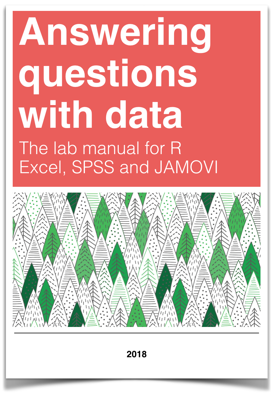
Chapter 6 Lab 3: Correlation
If … we choose a group of social phenomena with no antecedent knowledge of the causation or absence of causation among them, then the calculation of correlation coefficients, total or partial, will not advance us a step toward evaluating the importance of the causes at work. —Sir Ronald Fisher
In lecture and in the textbook, we have been discussing the idea of correlation. This is the idea that two things that we measure can be somehow related to one another. For example, your personal happiness, which we could try to measure say with a questionnaire, might be related to other things in your life that we could also measure, such as number of close friends, yearly salary, how much chocolate you have in your bedroom, or how many times you have said the word Nintendo in your life. Some of the relationships that we can measure are meaningful, and might reflect a causal relationship where one thing causes a change in another thing. Some of the relationships are spurious, and do not reflect a causal relationship.
In this lab you will learn how to compute correlations between two variables in software, and then ask some questions about the correlations that you observe.
6.1 General Goals
- Compute Pearson’s r between two variables using software
- Discuss the possible meaning of correlations that you observe
6.1.1 Important Info
We use data from the World Happiness Report. A .csv of the data can be found here: WHR2018.csv
6.2 R
In this lab we use explore to explore correlations between any two variables, and also show how to do a regression line. There will be three main parts. Getting r to compute the correlation, and looking at the data using scatter plots. We’ll look at some correlations from the World Happiness Report. Then you’ll look at correlations using data we collect from ourselves. It will be fun.
6.2.1 cor for correlation
R has the cor function for computing Pearson’s r between any two variables. In fact this same function computes other versions of correlation, but we’ll skip those here. To use the function you just need two variables with numbers in them like this:
x  <- c(1,3,2,5,4,6,5,8,9)
y  <- c(6,5,8,7,9,7,8,10,13)
cor(x,y)
## [1] 0.76539Well, that was easy.
6.2.1.1 scatterplots
Let’s take our silly example, and plot the data in a scatter plot using ggplot2, and let’s also return the correlation and print it on the scatter plot. Remember, ggplot2 wants the data in a data.frame, so we first put our x and y variables in a data frame.
library(ggplot2)

# create data frame for plotting
my_df <- data.frame(x,y)

# plot it
ggplot(my_df, aes(x=x,y=y))+
  geom_point()+
  geom_text(aes(label = round(cor(x,y), digits=2), y=12, x=2 ))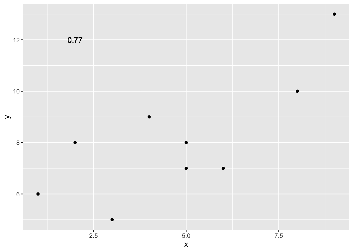
Wow, we’re moving fast here.
6.2.1.2 lots of scatterplots
Before we move on to real data, let’s look at some fake data first. Often we will have many measures of X and Y, split between a few different conditions, for example, A, B, C, and D. Let’s make some fake data for X and Y, for each condition A, B, C, and D, and then use facet_wrapping to look at four scatter plots all at once
x<-rnorm(40,0,1)
y<-rnorm(40,0,1)
conditions<-rep(c("A","B","C","D"), each=10)

all_df <- data.frame(conditions, x, y)

ggplot(all_df, aes(x=x,y=y))+
  geom_point()+
  facet_wrap(~conditions)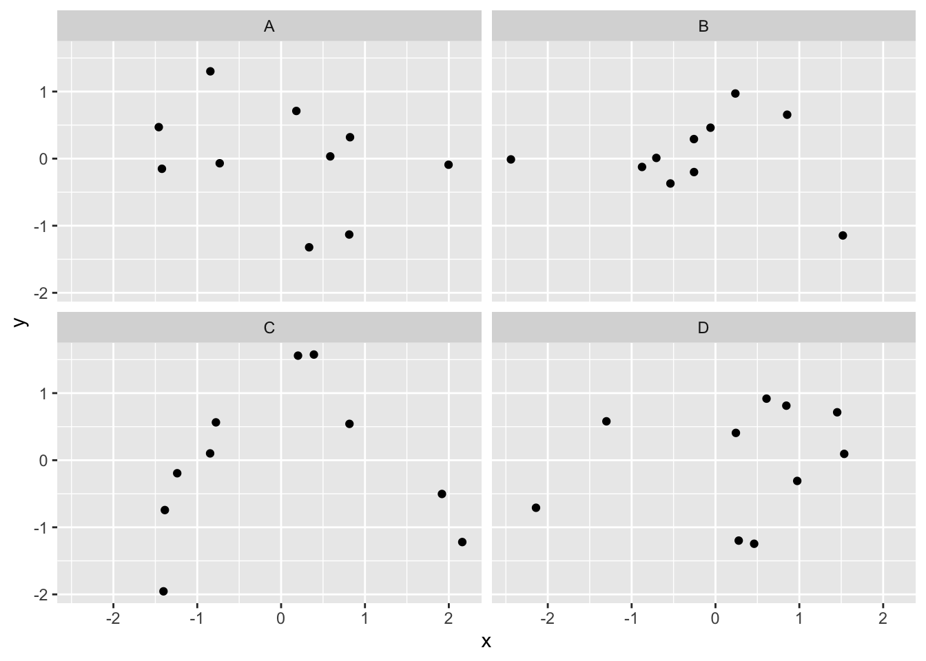
6.2.1.3 computing the correlations all at once
We’ve seen how we can make four graphs at once. Facet_wrap will always try to make as many graphs as there are individual conditions in the column variable. In this case there are four, so it makes four.
Notice, the scatter plots don’t show the correlation (r) values. Getting these numbers on there is possible, but we have to calculate them first. We’ll leave it to you to Google how to do this, if it’s something you want to do. Instead, what we will do is make a table of the correlations in addition to the scatter plot. We again use dplyr to do this:
OK, we are basically ready to turn to some real data and ask if there are correlations between interesting variables…You will find that there are some… But before we do that, we do one more thing. This will help you become a little bit more skeptical of these “correlations.”
6.2.1.4 Chance correlations
As you learned from the textbook. We can find correlations by chance alone, even when there is no true correlation between the variables. For example, if we sampled randomly into x, and then sampled some numbers randomly into y. We know they aren’t related, because we randomly sampled the numbers. However, doing this creates some correlations some of the time just by chance. You can demonstrate this to yourself with the following code. It’s a repeat of what we already saw, jut with a few more conditions added. Let’s look at 20 conditions, with random numbers for x and y in each. For each, sample size will be 10. We’ll make the fake data, then make a big graph to look at all. And, even though we get to regression later in the lab, I’ll put the best fit line onto each scatter plot, so you can “see the correlations.”
x<-rnorm(10*20,0,1)
y<-rnorm(10*20,0,1)
conditions<-rep(1:20, each=10)

all_df <- data.frame(conditions, x, y)

ggplot(all_df, aes(x=x,y=y))+
  geom_point()+
  geom_smooth(method=lm, se=FALSE)+
  facet_wrap(~conditions)+
  theme_classic()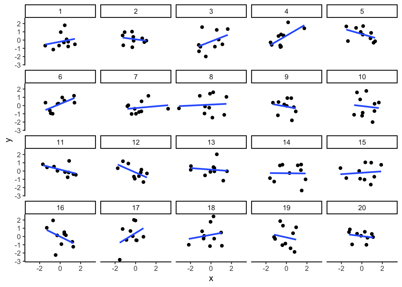
You can see that the slope of the blue line is not always flat. Sometimes it looks like there is a correlation, when we know there shouldn’t be. You can keep re-doing this graph, by re-knitting your r Markdown document, or by pressing the little green play button. This is basically you simulating the outcomes as many times as you press the button.
The point is, now you know you can find correlations by chance. So, in the next section, you should always wonder if the correlations you find reflect meaningful association between the x and y variable, or could have just occurred by chance.
6.2.2 World Happiness Report
Let’s take a look at some correlations in real data. We are going to look at responses to a questionnaire about happiness that was sent around the world, from the world happiness report
6.2.2.1 Load the data
We load the data into a data frame. Reminder, the following assumes that you have downloaded the RMarkdownsLab.zip file which contains the data file in the data folder.
library(data.table)
whr_data <- fread('data/WHR2018.csv')
You can also load the data using the following URL
library(data.table)
whr_data <- fread("https://raw.githubusercontent.com/CrumpLab/statisticsLab/master/data/WHR2018.csv")
6.2.2.2 Look at the data
library(summarytools)
view(dfSummary(whr_data))
You should be able to see that there is data for many different countries, across a few different years. There are lots of different kinds of measures, and each are given a name. I’ll show you some examples of asking questions about correlations with this data, then you get to ask and answer your own questions.
6.2.2.3 My Question #1
For the year 2017 only, does a country’s measure for “Freedom to make life choices” correlate with that country’s measure for " Confidence in national government"?
Let’s find out. We calculate the correlation, and then we make the scatter plot.
cor(whr_data$`Freedom to make life choices`,
    whr_data$`Confidence in national government`)
## [1] NAggplot(whr_data, aes(x=`Freedom to make life choices`,
y=`Confidence in national government`))+
geom_point()+
theme_classic()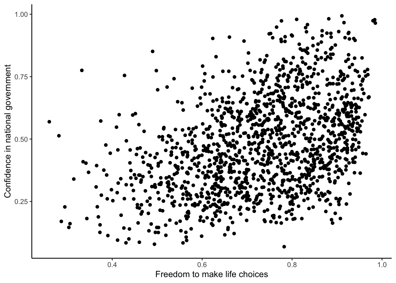
Interesting, what happened here? We can see some dots, but the correlation was NA (meaning undefined). This occurred because there are some missing data points in the data. We can remove all the rows with missing data first, then do the correlation. We will do this a couple steps, first creating our own data.frame with only the numbers we want to analyse. We can select the columns we want to keep using select. Then we use filter to remove the rows with NAs.
library(dplyr)

smaller_df <- whr_data %>%
               select(country,
                      `Freedom to make life choices`,
                      `Confidence in national government`) %>%
               filter(!is.na(`Freedom to make life choices`),
                      !is.na(`Confidence in national government`))

cor(smaller_df$`Freedom to make life choices`,
    smaller_df$`Confidence in national government`)
## [1] 0.4080963Now we see the correlation is .408.
Although the scatter plot shows the dots are everywhere, it generally shows that as Freedom to make life choices increases in a country, that country’s confidence in their national government also increase. This is a positive correlation. Let’s do this again and add the best fit line, so the trend is more clear, we use geom_smooth(method=lm, se=FALSE). I also change the alpha value of the dots so they blend it bit, and you can see more of them.
# select DVs and filter for NAs

smaller_df <- whr_data %>%
               select(country,
                      `Freedom to make life choices`,
                      `Confidence in national government`) %>%
               filter(!is.na(`Freedom to make life choices`),
                      !is.na(`Confidence in national government`))

# calcualte correlation

cor(smaller_df$`Freedom to make life choices`,
    smaller_df$`Confidence in national government`)
## [1] 0.4080963# plot the data with best fit line
ggplot(smaller_df, aes(x=`Freedom to make life choices`,
y=`Confidence in national government`))+
geom_point(alpha=.5)+
geom_smooth(method=lm, se=FALSE)+
theme_classic()
6.2.2.4 My Question #2
After all that work, we can now speedily answer more questions. For example, what is the relationship between positive affect in a country and negative affect in a country. I wouldn’t be surprised if there was a negative correlation here: when positive feelings generally go up, shouldn’t negative feelings generally go down?
To answer this question, we just copy paste the last code block, and change the DVs to be Positive affect, and Negative affect
# select DVs and filter for NAs

smaller_df <- whr_data %>%
               select(country,
                      `Positive affect`,
                      `Negative affect`) %>%
               filter(!is.na(`Positive affect`),
                      !is.na(`Negative affect`))

# calcualte correlation

cor(smaller_df$`Positive affect`,
    smaller_df$`Negative affect`)
## [1] -0.3841123# plot the data with best fit line
ggplot(smaller_df, aes(x=`Positive affect`,
y=`Negative affect`))+
geom_point(alpha=.5)+
geom_smooth(method=lm, se=FALSE)+
theme_classic()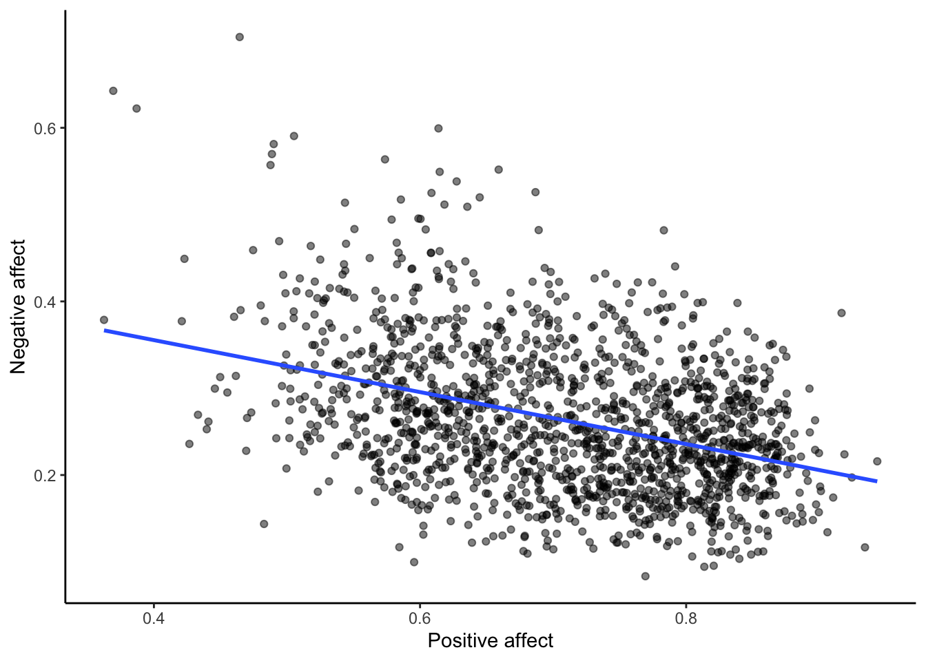
Bam, there we have it. As positive affect goes up, negative affect goes down. A negative correlation.
6.2.3 Generalization Exercise
This generalization exercise will explore the idea that correlations between two measures can arise by chance alone. There are two questions to answer. For each question you will be sampling random numbers from uniform distribution. To conduct the estimate, you will be running a simulation 100 times. The questions are:
Estimate the range (minimum and maximum) of correlations (using pearons’s r) that could occur by chance between two variables with n=10.
Estimate the range (minimum and maximum) of correlations (using pearons’s r) that could occur bychance between two variables with n = 100.
Use these tips to answer the question.
Tip 1: You can use the runif() function to sample random numbers between a minimum value, and maximum value. The example below sample 10 (n=10) random numbers between the range 0 (min = 0) and 10 (max=10). Everytime you run this code, the 10 values in x will be re-sampled, and will be 10 new random numbers
x <- runif(n=10, min=0, max=10)Tip 2: You can compute the correlation between two sets of random numbers, by first sampling random numbers into each variable, and then running the cor() function.
x <- runif(n=10, min=0, max=10)
y <- runif(n=10, min=0, max=10)
cor(x,y)
## [1] -0.6526973Running the above code will give different values for the correlation each time, because the numbers in x and y are always randomly different. We might expect that because x and y are chosen randomly that there should be a 0 correlation. However, what we see is that random sampling can produce “fake” correlations just by chance alone. We want to estimate the range of correlations that chance can produce.
Tip 3: One way to estimate the range of correlations that chance can produce is to repeat the above code many times. For example, if you ran the above code 100 times, you could save the correlations each time, then look at the smallest and largest correlation. This would be an estimate of the range of correlations that can be produced by chance. How can you repeat the above code many times to solve this problem?
We can do this using a for loop. The code below shows how to repeat everything inside the for loop 100 times. The variable i is an index, that goes from 1 to 100. The saved_value variable starts out as an empty variable, and then we put a value into it (at index position i, from 1 to 100). In this code, we put the sum of the products of x and y into the saved_value variable. At the end of the simulation, the save_value variable contains 100 numbers. The min() and max() functions are used to find the minimum and maximum values for each of the 100 simulations. You should be able to modify this code by replacing sum(x*y) with cor(x,y). Doing this will allow you to run the simulation 100 times, and find the minimum correlation and maximum correlation that arises by chance. This will be estimate for question 1. To provide an estimate for question 2, you will need to change n=10 to n=100.
saved_value <- c() #make an empty variable
for (i in 1:100){
  x <- runif(n=10, min=0, max=10)
  y <- runif(n=10, min=0, max=10)
  saved_value[i] <- sum(x*y)
}

min(saved_value)
## [1] 85.73592max(saved_value)## [1] 483.72756.2.4 Writing assignment
Answer the following questions with complete sentences. When you have finished everything. Knit the document and hand in your stuff (you can submit your .RMD file to blackboard if it does not knit.)
Imagine a researcher found a positive correlation between two variables, and reported that the r value was +.3. One possibility is that there is a true correlation between these two variables. Discuss one alternative possibility that would also explain the observation of +.3 value between the variables.
Explain the difference between a correlation of r = .3 and r = .7. What does a larger value of r represent?
Explain the difference between a correlation of r = .5, and r = -.5.
6.3 Excel
How to do it in Excel
6.4 SPSS
In this lab, we will use SPSS to calculate the correlation coefficient. We will focus on the most commonly used Pearson’s coefficient, r. We will learn how to:
- Calculate the Pearson’s r correlation coefficient for bivariate data
- Produce a correlation matrix, reporting Pearson’s r for more than two variables at a time
- Produce a scatterplot
- Split a data file for further analysis
Let’s first begin with a short data set we will enter into a new SPSS data spreadsheet. Remember, in order to calculate a correlation, you need to have bivariate data; that is, you must have at least two variables, x and y. You can have more than two variables, in which case we can calculate a correlation matrix, as indicated in the section that follows.
6.4.1 Correlation Coefficient for Bivariate Data: Two Variables
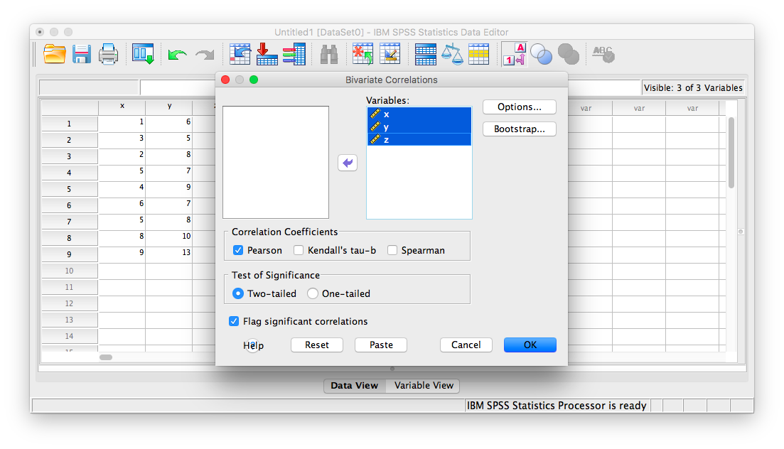
Let’s use the following data set: {x= 1, 3, 2, 5, 4, 6, 5, 8, 9} {y= 6, 5, 8, 7, 9, 7, 8, 10, 13}. Notice there are two variables, x and y. Enter these into SPSS and name them appropriately.
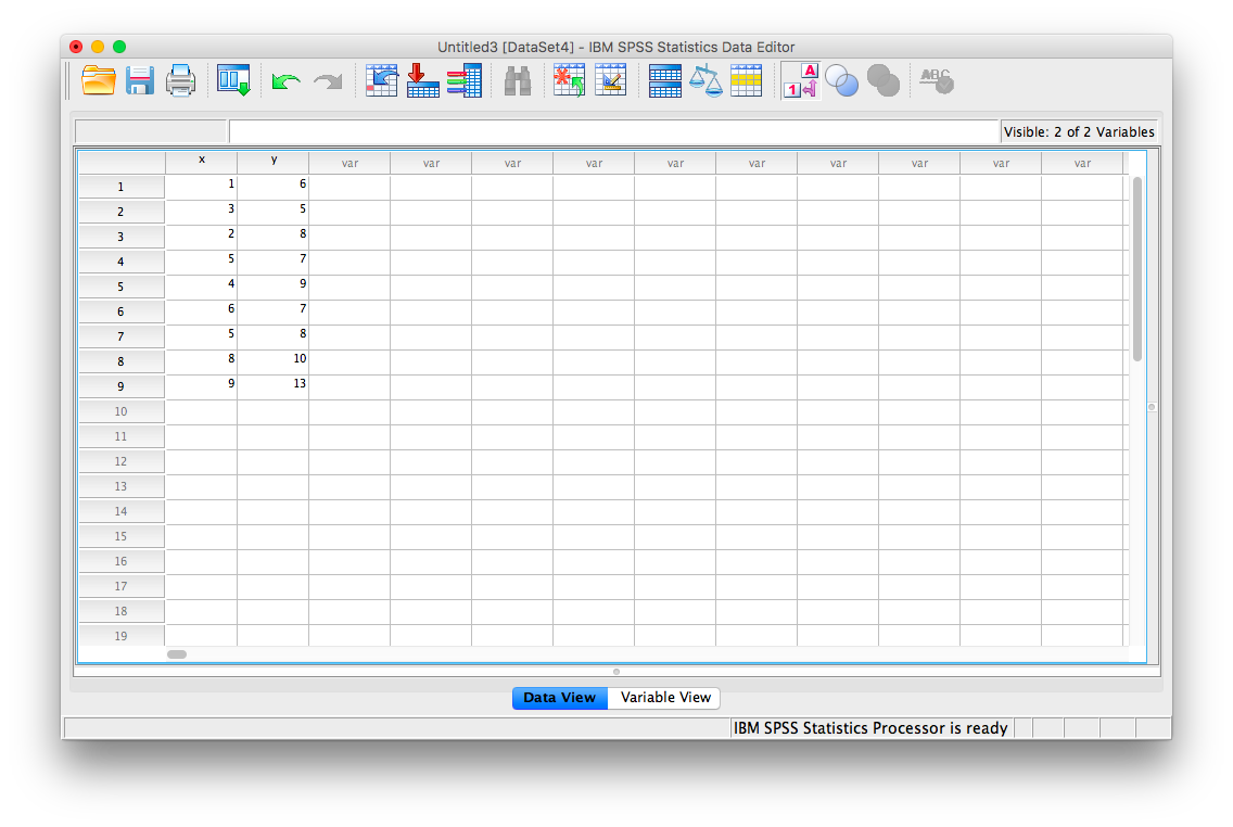
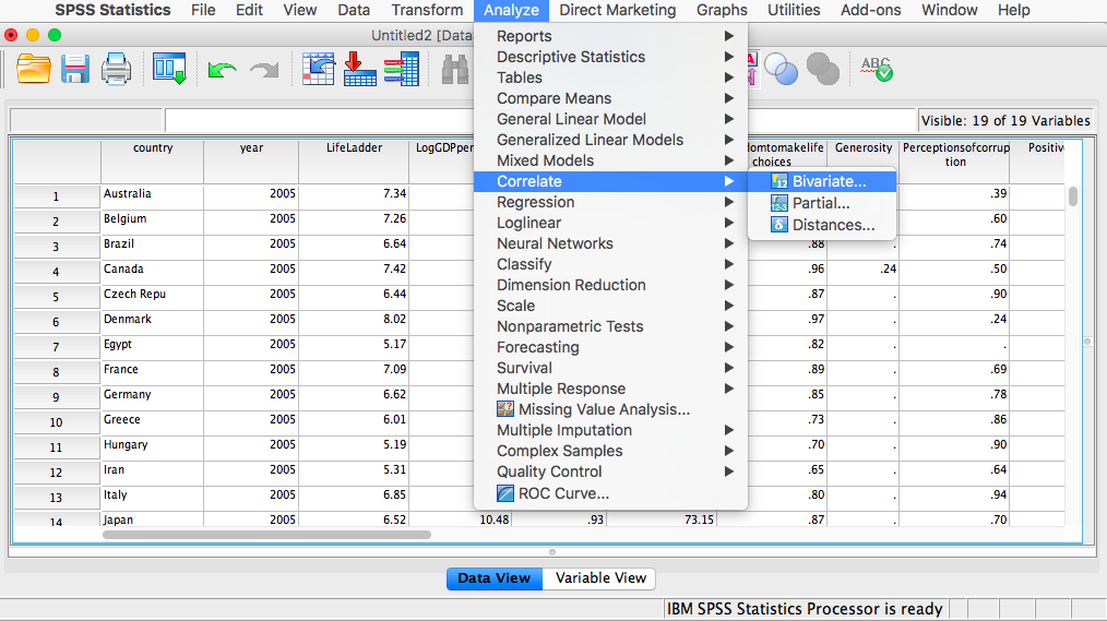
Next, click Analyze, then Correlate, then Bivariate:

The next window will ask you to select variables to correlate. Since we have two (x and y) move them both from the left-hand field to the right-hand field using the arrow. Notice that in this window, Pearson is selected. This is the default setting (and the one we want), but notice there are other ways to calculate the correlation between variables. We will stick with Pearson’s correlation coefficient for this course.
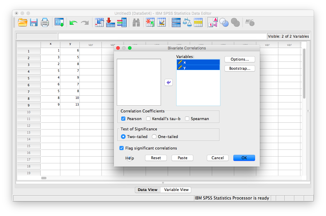
Now, click OK.
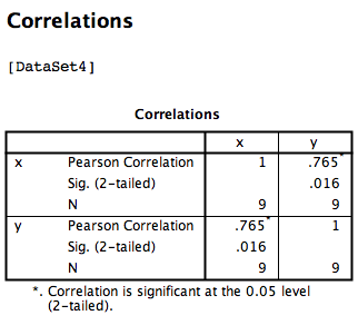
SPSS will produce an output table containing the correlation coefficient requested. Notice that the table is redundant; it gives us the correlation between x and y, the correlation between y and x, the correlation between x and itself, and the correlation between y and itself. Any variable correlated with itself will result in an r of 1. The Pearson r correlation between variables x and y is .765.
6.4.2 Correlation Matrix
In the event that you have more than two variables in your spreadsheet, and would like to evaluate correlations between several variables taken two at a time, you need not re-run the correlations in SPSS repeatedly. You can, in fact, enter multiple variables into the correlation window and obtain a correlation matrix–a table showing every possible bivariate correlation amongst a group of variables.
To illustrate how this is done, let’s add a new variable to our existing spreadsheet: variable z, {z= 1, 4, 2, 9, 5, 7, 12, 5, 3}
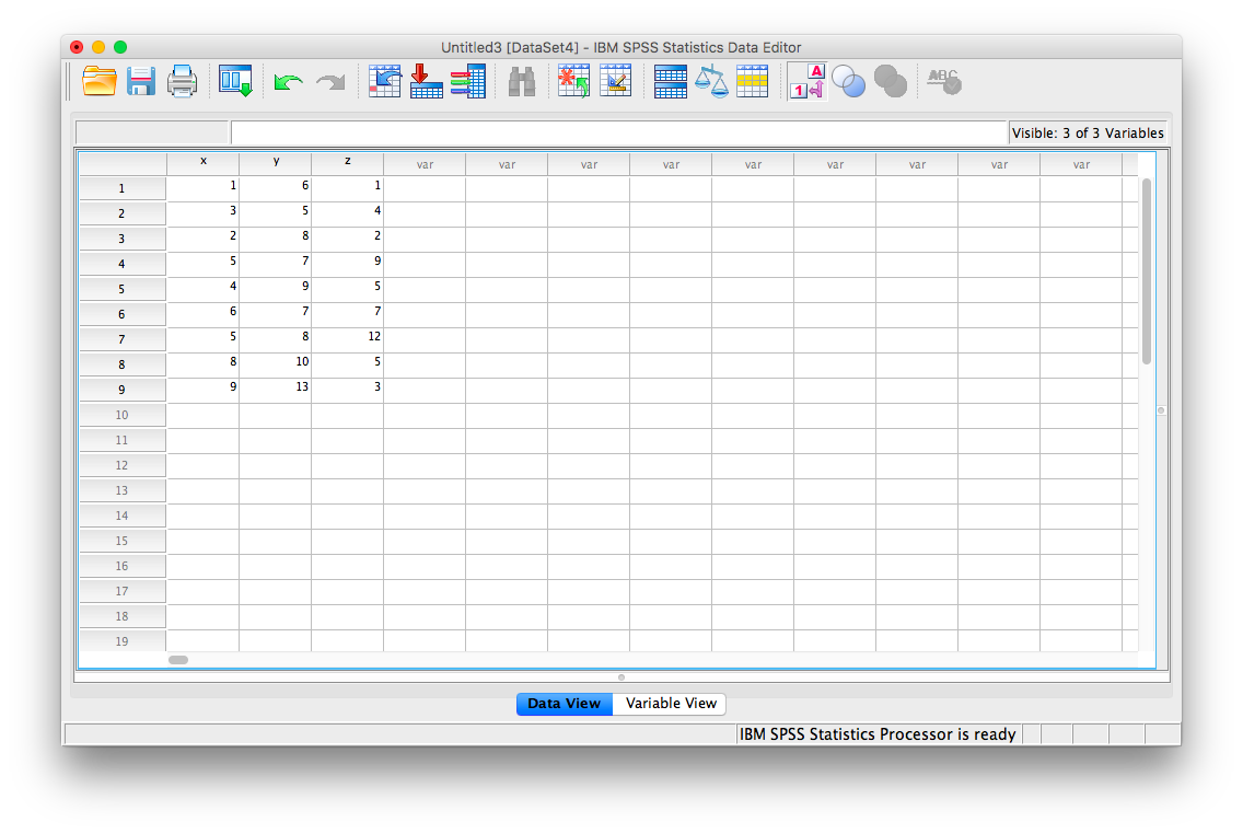
From here, go to Analyze, then Correlate, then Bivariate:
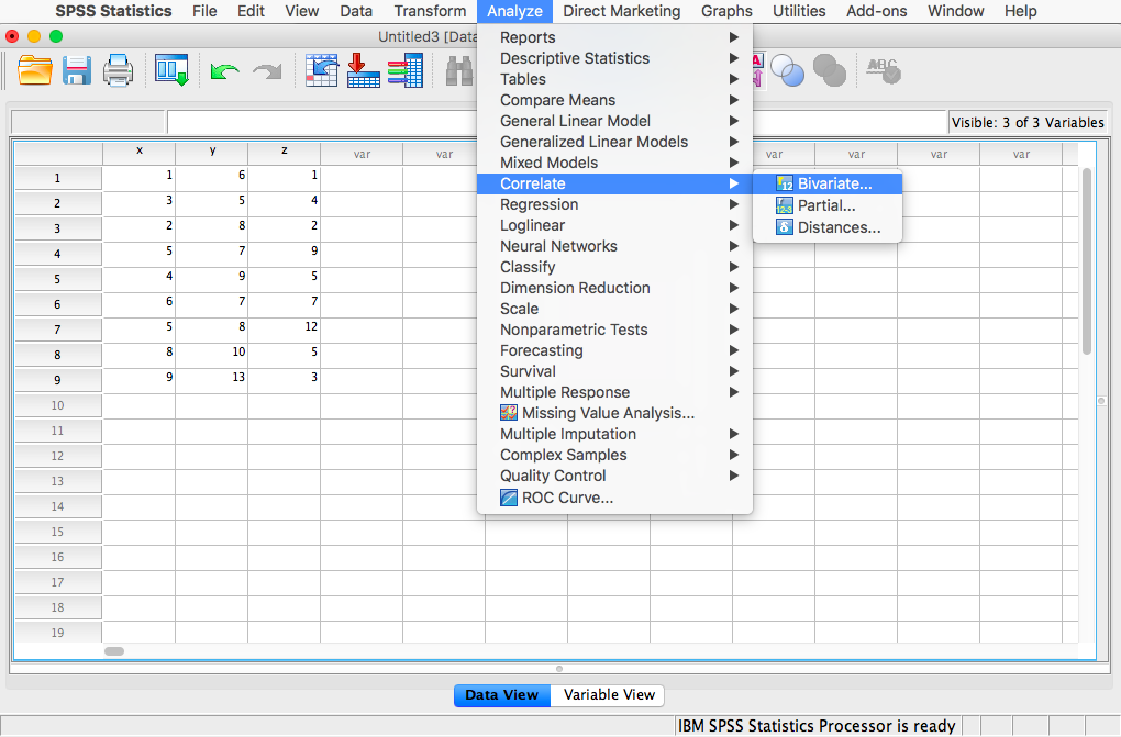
Next, you will encounter the window that asks you to indicate which variables to correlate. Select all three variables (x, y, and z) and move them to the right-hand field using the arrow.
Click OK. SPSS will produce an output table that contains correlations for every pairing of our three variables, along with the correlations of each variable with itself.
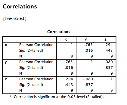
According to this output:
- The correlation coefficient between variables
xandyis .765 - The correlation coefficient between variables
xandzis .294 - The correlation coefficient between variables
yandzis -.080
6.4.3 Correlation and Scatterplots
To accompany the calculation of the correlation coefficient, the scatterplot is the relevant visualization tool. Let’s use data from The World Happiness Report, a questionnaire about happiness. Here is a link to the file named WHR2018.sav.
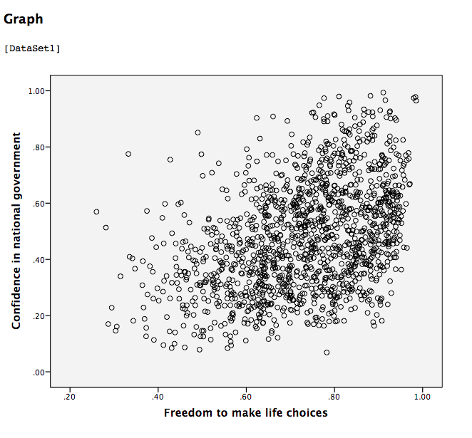
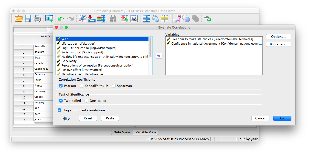
Using this data, let’s answer the following question: does a country’s measure for Freedom to make life choices correlate with that country’s measure for Confidence in national government?
Let’s find the correlation coefficient between these variables first. Go to Analyze, then Correlate, then Bivariate:
Next, a window will appear asking for the variables to be correlated. Go through the list on the left and find Freedom to make life choices as well as Confidence in national government. Move both of these variables to the field on the right using the arrow.
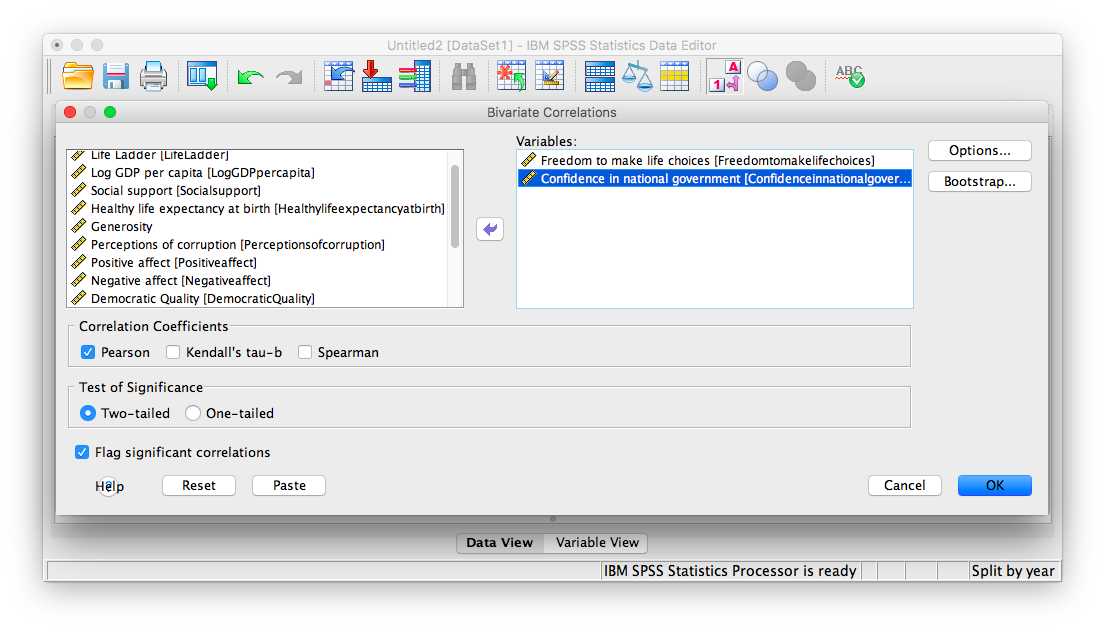 Click OK. SPSS will produce a correlation table.
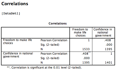
Based on this output, the correlation between Freedom to make life choices and Confidence in national government is .408.
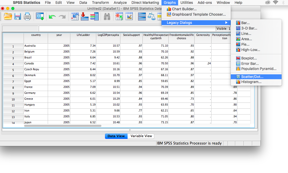
Let’s continue to create the scatterplot for this data. Go to Graphs, then Legacy Dialogs, then Scatter…
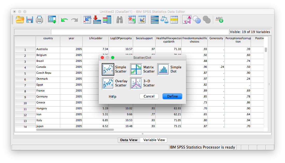
In the next window, choose Simple, then Define:
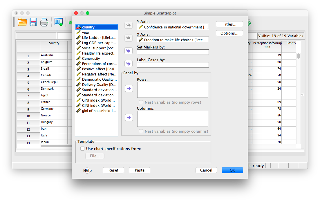
Next, move your two variables (Freedom to make life choices and Confidence in national government) into the x-axis and y-axis fields. Again, it does not matter which variable goes where, for now.
Click OK. SPSS will produce a scatterplot of your data, as follows:
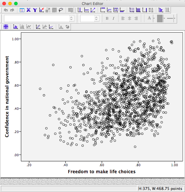
You can keep this scatterplot as it is, or, you can edit it to include a straight line that best fits the data points. This line is known as the best-fitting line as it minimizes the distance from it to all the data. To edit the scatterplot double click on the graph and a window labeled Chart Editor should appear:
In this window, find the button at the top that reads Fit Line at Total when you hover your mouse over it. Below, I have highlighted it for clarity:
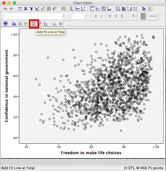
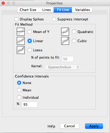
Press this button and you will see a new menu. Make sure Linear is selected and click Apply.
Next, exit from the Chart Editor. This means you will hit the X in the corner of the window. You will find that the graph in your output window has now updated and has a line drawn on it.
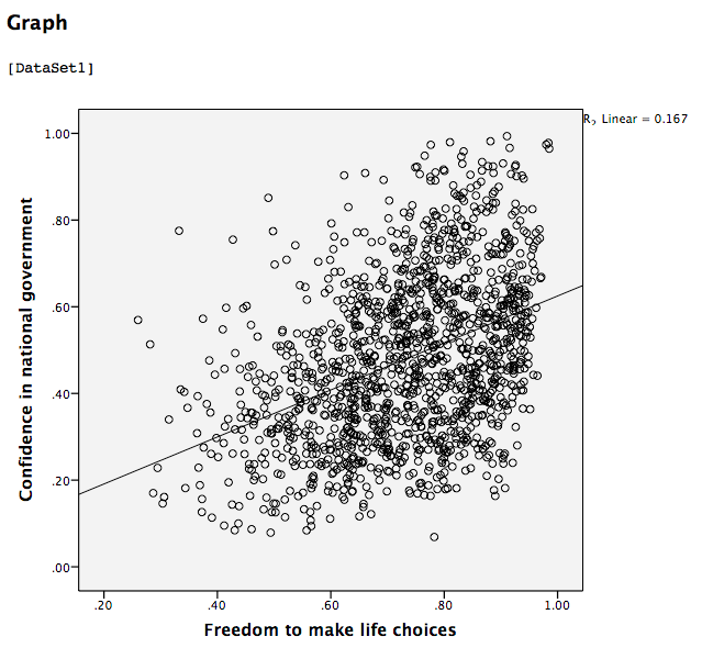
This scatterplot is very important. The distance between the line and the data points is indicative of the strength of the correlation coefficient; they are directly related. For example, if the data were more clustered or tighter to the line, the correlation would be stronger. If the data points are more spread out and far from the line, the correlation is weaker.
6.4.4 Splitting a File
What if we asked the question: for the year 2017 only, does a country’s measure for Freedom to make life choices correlate with that country’s measure for Confidence in national government?
Notice that this question is asking us to find the correlation between the same two variables we used in the previous example, but only in the case where the year is 2017. To acheive this, we’re going to utilize a function called splitting. Splitting takes the file as a whole, and sets it up so that every analysis is done on some subset of the data. For example, if we split our data by year and calculate a correlation coefficient, SPSS will find Pearson r for only 2017, and another for only 2016, and so on.
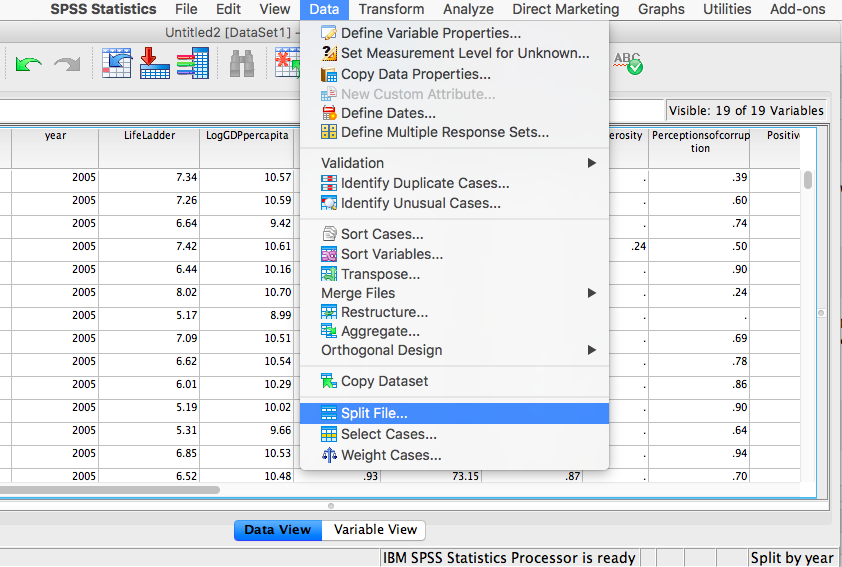
In order to split the data, we go to the top menu and choose Data, then Split file…
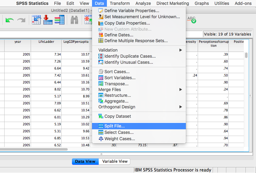
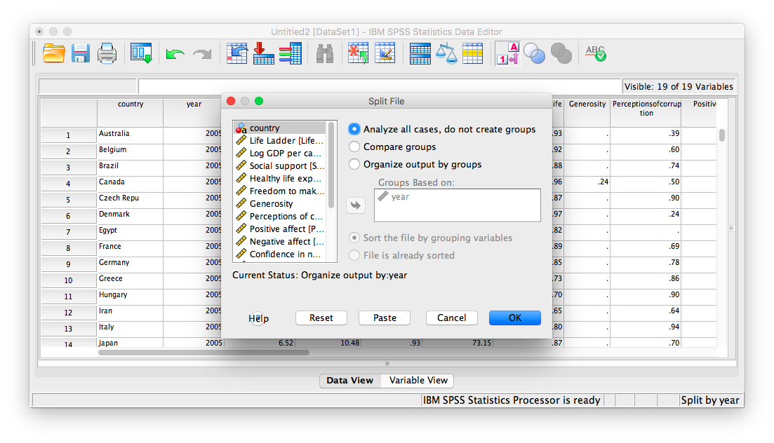
In the next window, you must select Organize output by groups and then specify which variable will be used to split the data. Select year and move it to the right-hand field using the arrow.
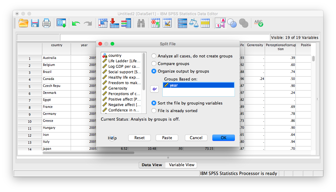
Click OK. Notice that this will cause the output window to produce some text indicating that you have split your file. You can ignore this and go back to your data window.
From here, any analysis you choose to do will be done separately for each year’s worth of data. Let’s calculate the correlation coefficient, as usual. Click Analyze, then Correlate, then Bivariate:
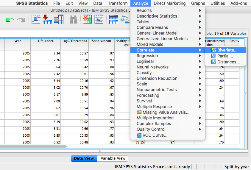
In the next window, select the variables to be used (they will be the same as in the last example).
Click OK. Notice that in the output window you will see a bunch of correlation tables (13 of them to be exact), one for each year. Scroll down and find the table with the heading “year = 2017.” That’s the table we need in order to answer our question:
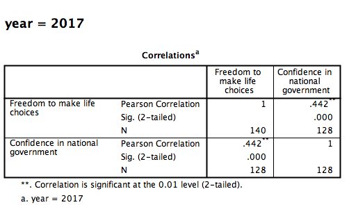
This table indicates that, if we only look at the year 2017, the correlation coefficient between Freedom to make life choices and Confidence in national government is .442.
It is VERY important to remember that once you have split a file, every analysis that follows the split will be done on the split variable. If you want to go back to performing analyses and calculating statistics for the data as a whole, you must UNSPLIT your data file (or undo the split). To do this, go to Data, then Split file…
Then make sure to select Analyze all cases, do not create groups and click OK.
6.4.5 Practice Problems
For the year 2005 ONLY, find the correlation between “perceptions of corruption” and “positive affect.” Create a scatterplot to visualize this relationship. What are your conclusions about the relationship between affect and perceived corruption? Is this surprising to you?
What has happened to log GDP (consider this a measure of GDP) in the United States ONLY with time (as the year has increased)? Explain this relationship and provide a scatterplot.
Which country (or countries) have seen a more consistent and strong increase in log GDP over time? Which country (or countries) have seen a decrease over time?
6.5 JAMOVI
This section is copied almost verbatim, with some editorial changes, from Answering questions with data: The lab manual for R, Excel, SPSS and JAMOVI, Lab 3, Section 3.4, SPSS, according to its CC license. Thank you to Crump, Krishnan, Volz, & Chavarga (2018).
In this lab, we will use jamovi to calculate the correlation coefficient. We will focus on the most commonly used Pearson’s coefficient, r. We will learn how to:
- Calculate the Pearson’s r correlation coefficient for bivariate data
- Produce a correlation matrix, reporting Pearson’s r for more than two variables at a time
- Produce a scatterplot
- Applying a filter to the data set for further analysis
Let’s first begin with a short data set we will enter into a new jamovi data spreadsheet. Remember, in order to calculate a correlation, you need to have bivariate data; that is, you must have at least two variables, x and y. You can have more than two variables, in which case we can calculate a correlation matrix, as indicated in the section that follows.
6.5.1 Correlation Coefficient for Bivariate Data: Two Variables
Let’s use the following data set: {x= 1, 3, 2, 5, 4, 6, 5, 8, 9} {y= 6, 5, 8, 7, 9, 7, 8, 10, 13}. Notice there are two variables, x and y. Enter these into jamovi, name them appropriately, and be sure to indicate, in the Analyze, that these data are measured on a continuous scale. (REMEMBER: One assumption of Pearson’s correlation is that the variables are measured on at least an interval scale. That means you should not use Pearson’s correlation with variables that are measured on an ordinal scale. Spearman’s correlation may be helpful if you have variables measured on an ordinal scale.)
Remember to use the upward facing arrow or the Settings button to close the Analyze pop-up window.
Next, click Analyses, Regression, and Correlation Matrix:
In the pop-up window, you will select variables to correlate. Since we have two (x and y) move them both from the left-hand field to the right-hand field by highlighting them and using the arrow. Notice that in this window, Pearson is selected. This is the default setting (and the one we want), but notice there are other ways to calculate the correlation between variables. We will stick with Pearson’s correlation coefficient for now.
In the Results panel on the left, jamovi will produce an output table containing the correlation coefficient requested. (If you are familiar with SPSS, you may notice that the jamovi table is unlike the SPSS table in that the jamovi correlation matrix does not have the redundant information in the top and bottom triangles of the matrix; jamovi gives us only the correlation between x and y in the bottom portion of the table. Note: Any variable correlated with itself will result in an r of 1.) The Pearson r correlation between variables x and y is .765.
6.5.2 Correlation Matrix
In the event that you have more than two variables in your spreadsheet, and would like to evaluate correlations between several variables taken two at a time, you need not re-run the correlations in jamovi repeatedly. You can, in fact, enter multiple variables into the correlation window and obtain a correlation matrix–a table showing every possible bivariate correlation amongst a group of variables.
To illustrate how this is done, let’s add a new variable to our existing spreadsheet: variable z, {z= 1, 4, 2, 9, 5, 7, 12, 5, 3}.
From here, go to Analyses, then Regression, and then Correlation Matrix:
Next, you will encounter the window that asks you to indicate which variables to correlate. Select all three variables (x, y, and z) by highlighting them, and move them to the right-hand field using the arrow.
jamovi will produce an output table in the Results panel to the right that contains correlations for every pairing of our three variables. You should see three correlation coefficients and three associated p-values.
According to this output:
- The correlation coefficient between variables
xandyis .765; that is, Pearson’s r for variablesxandyis .765. - The correlation coefficient between variables
xandzis .294; Pearson’s r forxandzis .294. - The correlation coefficient between variables
yandzis -.080; Pearson’s r foryandzis -.080.
To further our understanding of these correlation coefficients, we should also look to the p-values associated with each coefficient to decide if the correlation is significant or non-significant.
- Pearson’s r for variables
xandyis .765. The p-value is .02 which is less than a conventional alpha level of .05, so we would consider this result to be significant. We might write: A Pearson’s correlation was performed, and variablesxandywere found to be significantly correlated, r = .77, p = .02. - Pearson’s r for
xandzis .294. The p-value is .44 which is greater than a conventional alpha level of .05, so we would consider this result to be non-significant. We might write: A Pearson’s correlation was performed, and no significant correlation was found between variablesxandz, r = .29, p > .05. - Pearson’s r for
yandzis -.080. The p-value is .84 which is greater than a conventional alpha level of .05, so we would consider this result to be non-significant. We might write: A Pearson’s correlation was performed, and no significant correlation was found between variablesyandz, r = -.08, p > .05.
6.5.3 Correlation and Scatterplots
To accompany the calculation of the correlation coefficient, the scatterplot is the relevant visualization tool. Let’s use data from EngageNS.
Using this data, let’s answer the following question: Does Number of hours per week spent working at main job correlate with Home activity participation on a typical day: Playing computer games?
Let’s find the correlation coefficient between these variables first. Go to Analyses, then Regression, and then Correlation Matrix:
Next, a window will appear asking for the variables to be correlated. Use the search function to speed up your identification of those variables. Rather than scrolling through all of the variables in the list on the left, look into the Data Dictionary to find the variable names and search for them. Move both of these variables to the field on the right using the arrow.
In the Results panel, jamovi will produce a correlation table.
Based on this output, the correlation between WORKHR and HM_CGAME is -.042. The negative sign simply indicates that as the scores on one variable increase, the scores on the other variable decrease; the variables are negatively correlated. Looking at the p-value, we see it is .001, which is less than our commonly used alpha levels. This correlation is significant.
We might communicate this information like this: A Pearson’s correlation analysis was performed, and a significant negative correlation was found between Number of hours per week spent working at main job and Home activity participation on a typical day: Playing computer games, r = -.04, p = .001.
6.5.3.1 Adding the Scatterplot module to jamovi
Before you can request a scatterplot in jamovi, you must add Scatterplot as a module. To do so, click on the addition sign which is white with a blue trim that has the word “Modules” under the sign. Click jamovi library. Under the “Available” tab, you should see a module called scatr. Click to INSTALL it. When it is installed, it will appear in your Exploration menu.
6.5.3.2 Getting a visual of the correlation
Let’s continue to create the scatterplot for this data.
Go to Analyses, then Exploration, and then Scatterplot.
In the next window, choose Simple, then Define:
Next, move your two variables (WORKHR and HM_CGAMES) into the x-axis and y-axis fields. Again, it does not matter which variable goes where, for now. (Remember to use the search function to speed up your search for the variables to include.)
In the Results panel, jamovi will produce a scatterplot of your data, as follows:
You can keep this scatterplot as it is, or, you can edit it to include a straight line that best fits the data points. This line is known as the best-fitting line as it minimizes the distance from it to all the data. To include the line of best fit, click on Linear under the Regression Line heading.
You will find that the graph in your Results panel has now updated and has a line drawn on it.
This line of best fit on the scatterplot is barely visible. Typically, the distance between the line and the data points is indicative of the strength of the correlation coefficient; they are directly related. For example, if the data were more clustered or tighter to the line, the correlation would be stronger. If the data points are more spread out and far from the line, the correlation is weaker. In this case, although there are many data points clustered around the line, we also see there are a number of data points that are quite far from the line. This is a moderate correlation. We also see that this negative correlation is depicted by a line that falls to the left (i.e., a line with a negative slope).
6.5.4 Applying a Filter
What if we asked the question: For residents of the Antigonish and Guysborough regions only, does Number of hours per week spent working at main job correlate with Home activity participation on a typical day: Playing computer games?
Notice that this question is asking us to find the correlation between the same two variables we used in the previous example, but only in the case where the REGION is equal to 4. To achieve this, we’re going to utilize a function called filtering. Filtering the data set makes only those cases that meet our criteria available for use in the analysis to be run. For example, if we filter our data by region and calculate a correlation coefficient, jamovi will find Pearson r for only Antigonish and Guysborough, and not for other regions.
In order to filter the data, we go to the top menu and choose Data and then Filter.
In the next window, you must set up the filter; indicate which cases will be used. Under “Filter 1,” click on the formula editor, the fx button. Double click on the variable name (REGION), and it will be incorporated into the filter. Then, use two equal signs, and enter the code for the region of interest (4).
Notice that this will cause a new column in the spreadsheet wherein a green checkmark indicates the case/participant will be included in the analysis and a red “x” indicates the case/participant will be excluded from the analysis.
From here, any analysis you choose to do will be done for only the cases match the filter. Let’s calculate the correlation coefficient, as usual. Click Analyses, then Regression, and then Correlation Matrix:
In the next window, select the variables to be used (they will be the same as in the last example).
Notice that in the output now shows a correlation matrix with different results than you saw when you ran the correlation with the entire data set:
This table indicates that, if we only look at the Antigonish-Guysborough region, the correlation coefficient between between WORKHR and HM_CGAME is .012 and the p-value is .80. Comparing this p-value to an alpha level of .05, we would say this correlation is non-significant.
Again, you may want to inspect the scatterplot to get a visual representation of this correlation coefficient for the data collected from participants in the Antigonish-Guysborough region. Challenge: Give the creation of this scatterplot a try on your own. See if your graph matches the one depicted below.
6.5.5 Removing the Filter
It is VERY important to remember that once you have applied a filter, every analysis will be done on the split variable. If you want to go back to performing analyses and calculating statistics for the data as a whole, you must delete the filter. To do this, you can highlight the column showing the filter in the spreadsheet, go to Data, and then Delete. You will be prompted with a question to verify that you want to delete the filter. Click Yes.
6.5.6 Homework
Look at participants’ reported number of close friends and their reported time spent socializing with friends. Are these scores correlated? If so, report r and whether the correlation is significant or non-signifcant?
Apply a filter so that you are looking at only the data for participants’ whose main activity is going to school (Hint: Use the data dictionary to figure out how participants’ main activities were coded.). Now, run the same correlation you looked at in #1. Are number of close friends and reported time spent socializing with friends correlated for students? Is the correlation significant? Compare these results to the results in #1. Is the correlation between number of close friends and reported time spent socializing with friends stronger or weaker for students than it is for Nova Scotians?
6.5.7 Practice Problems
Use the EngageNS data to answer the following questions:
Construct a scatterplot using FRIENDS on the x-axis and SOC_FRND on the y-axis to depict the results you found for the last homework question.
Can you run a Pearson’s correlation analysis on the following pairs of variables? Why or why not?
- SEX and SLEEP?
- COMP_TIME and SLEEP?
- MAINACT and EDUCAT?
- Run the correlation analysis for any set(s) of variables you determined to be appropriate for using Pearson’s correlation. Report the correlation coefficient. Is it considered statistically significant? Write your results following the APA rules discussed below.
Some formatting guidelines for writing results sections:
All of the numbers are rounded to two decimal places, but if your p-value was .0001, it would be okay to write p < .001.
Italicize symbols such as p and t.
There are spaces on either side of =, >, or < symbols.
Construct the scatterplot for any set(s) of variables you determined to be appropriate for using Pearson’s correlation. What do you notice about the scatterplot? Does the slope increase or decrease? Do the dots closely follow the line of best fit?
TBD: questions based on PSYC 291 survey / may want to move some from Lab 7
The follwoing three questions are copied verbatim from Answering questions with data: The lab manual for R, Excel, SPSS and JAMOVI, Lab 3, Section 3.2.4, SPSS, according to its CC license. Thank you to Crump, Krishnan, Volz, & Chavarga (2018).
Imagine a researcher found a positive correlation between two variables, and reported that the r value was +.3. One possibility is that there is a true correlation between these two variables. Discuss one alternative possibility that would also explain the observation of +.3 value between the variables.
Explain the difference between a correlation of r = .3 and r = .7. What does a larger value of r represent?
Explain the difference between a correlation of r = .5, and r = -.5.